What is RocksDB?

RocksDB is an embeddable persistent key-value store for fast storage.

• High Performance: RocksDB uses a log structured database engine, written entirely in C++, for maximum performance. Keys and values are just arbitrarily-sized byte streams.

• Optimized for Fast Storage: RocksDB is optimized for fast, low latency storage such as flash drives and high-speed disk drives. RocksDB exploits the full potential of high read/write rates offered by flash or RAM.

• Adaptable: RocksDB is adaptable to different workloads. From database storage engines such as MyRocks to application data caching to embedded workloads, RocksDB can be used for a variety of data needs.

• Basic and Advanced Database Operations: RocksDB provides basic operations such as opening and closing a database, reading and writing to more advanced operations such as merging and compaction filters.

High Level Architecture

RocksDB is an embedded key-value store where keys and values are arbitrary byte streams. RocksDB organizes all data in sorted order and the common operations are Get(key), Put(key), Delete(key) and NewIterator().

The three basic constructs of RocksDB are memtable, sstfile (LSM) and logfile. The memtable is an in-memory data structure - new writes are inserted into the memtable and are optionally written to the logfile. The logfile is a sequentially-written file on storage. When the memtable fills up, it is flushed to a sstfile on storage and the corresponding logfile can be safely deleted. The data in an sstfile is sorted to facilitate easy lookup of keys.

Features

• RocksDB supports partitioning a database instance into multiple column families.
• A Put API inserts/overwrites a single key-value to the database; A Write API allows multiple keys-values to be atomically inserted into the database.
• Keys and values are treated as pure byte streams. There is no limit to the size of a key or a value. Get/MultiGet, Iterator and Snapshot.
• Prefix iterator, RocksDB can config a prefix_extractor to specify a key-prefix. An iterator that specifies a prefix will use these bloom bits to avoid looking into unwanted data file.
• RocksDB uses a checksum to detect corruptions in storage. These checksums are for each SST file block (typically between 4K to 128K in size)
• RocksDB supports snappy, zlib, bzip2, lz4, lz4_hc, and zstd compression.
• Full Backups, Incremental Backups and Replication.
• Block Cache – Compressed and Uncompressed Data, RocksDB uses a LRU cache for blocks to serve reads.
• The default implementation of the memtable for RocksDB is a skiplist. Three pluggable memtables are part of the library: a skiplist memtable, a vector memtable and a prefix-hash memtable.
• When a memtable is full, it becomes an immutable memtable and a background thread starts flushing its contents to storage. Meanwhile, new writes continue to accumulate to a newly allocated memtable.
• When a memtable is being flushed to storage, an inline-compaction process removes duplicate records from the output steam. When a compaction process encounters a Merge record, it invokes an application-specified method called the Merge Operator. The Merge can combine multiple Put and Merge records into a single one.

MemTable

MemTable is an in-memory data-structure holding data before they are flushed to SST files. Use an in-memory balanced tree data structure (red-black trees or AVL trees), sometimes called memtable, you can insert keys in any order and read them back in sorted order. When the memtable gets bigger than some threshold (typically a few megabytes), write it out to disk as an SSTable file. In order to serve a read request, first try to find the key in the memtable, then in the most recent on-disk segment, then in the next-older segment, etc. From time to time, run a merging and compaction process in the background to combine segment files and to discard overwritten or deleted values.

SST File

All RocksDB’s persistent data is stored in a collection of SSTs, Static Sorted Table. There are two types of tables: “plain table” and “block based table”.

In block based table, data is chunked into (almost) fixed-size blocks (4~128K). Each block keeps a bunch of entries.

When storing data, we can compress and/or encode data efficiently within a block, which often resulted in a much smaller data size compared with the raw data size.

As for the record retrieval, we’ll first locate the block where target record may reside, then read the block to memory, and finally search that record within the block. Of course, to avoid frequent reads of the same block, we introduced the block cache to keep the loaded blocks in the memory.

File Format

<beginning_of_file>
[data block 1]
[data block 2]
...
[data block N]
[meta block 1: filter block]                  (see section: "filter" Meta Block)
[meta block 2: stats block]                   (see section: "properties" Meta Block)
[meta block 3: compression dictionary block]  (see section: "compression dictionary" Meta Block)
[meta block 4: range deletion block]          (see section: "range deletion" Meta Block)
...
[meta block K: future extended block]  (we may add more meta blocks in the future)
[metaindex block]
[index block]
[Footer]                               (fixed size; starts at file_size - sizeof(Footer))
<end_of_file>

Block Cache

There are two cache implementations in RocksDB, namely LRUCache and ClockCache. Both types of the cache are sharded to mitigate lock contention. Capacity is divided evenly to each shard and shards don’t share capacity. By default each cache will be sharded into at most 64 shards, with each shard has no less than 512k bytes of capacity.

Synchronization is done via a per-shard mutex. Both lookup and insert to the cache would require a locking mutex of the shard. num_shard_bits: The number of bits from cache keys to be use as shard id. The cache will be sharded into 2^num_shard_bits shards. so that we can easily calculate shard id with bit operation ((1 « num_shard_bits) - 1 & key).

Column Families

Each key-value pair in RocksDB is associated with exactly one Column Family. If there is no Column Family specified, key-value pair is associated with Column Family “default”. Column Families provide a way to logically partition the database.

Compression Dictionary

The dictionary will be constructed by sampling the first output file in a subcompaction when the target level is bottommost. Samples are 64 bytes each and taken uniformly/randomly over the file. When picking sample intervals, we assume the output file will reach its maximum possible size.

Once generated, this dictionary will be loaded into the compression library before compressing/uncompressing each data block of subsequent files in the subcompaction. The dictionary is stored in the file’s meta-block in order for it to be known when uncompressing.

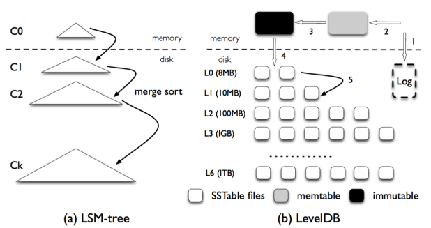
Leveled Compaction

LSM (Long Structured Merged) Tree is a data structure with performance characteristics that make it attractive for providing indexed access to files with high insert volume, such as transactional log data.

Files on disk are organized in multiple levels. We call them level-1, level-2, etc, or L1, L2, etc, for short. A special level-0 (or L0 for short) contains files just flushed from in-memory write buffer (memtable). Each level (except level 0) is one data sorted run. Inside each level (except level 0), data is range partitioned into multiple SST files.

To identify a position for a key, we first binary search the start/end key of all files to identify which file possibly contains the key, and then binary search inside the key to locate the exact position. In all, it is a full binary search across all the keys in the level.

Extensions to the ‘levelled’ method to incorporate B+ tree structures have been suggested.

LSM trees are used in data stores such as Bigtable, HBase, LevelDB, MongoDB, SQLite4[5], Tarantool [6], RocksDB, WiredTiger,[7] Apache Cassandra, and InfluxDB.

Cassandra

What is Cassandra?

“Apache Cassandra is an open source, distributed, decentralized, elastically scalable, highly available, fault-tolerant, tuneably consistent, row-oriented database that bases its distribution design on Amazon’s Dynamo and its data model on Google’s Bigtable. Created at Facebook, it is now used at some of the most popular sites on the Web.”

Cassandra addresses the problem of failures by using a peer-to-peer distributed system across homogeneous nodes where data is distributed among all nodes in the cluster. Each node exchanges information across the cluster every second (Gossip Protocol). A sequentially written commit log on each node captures write activity to ensure data durability. Data is then indexed and written to an in-memory structure (balanced tree), called a memtable, which resembles a write-back cache. Once the in-memory data structure is full, the data is written to disk in an SSTable data file. All writes are automatically partitioned and replicated throughout the cluster (Requests can wait to choose for one node, a quorum, or all nodes to accept the write). Using a process called compaction Cassandra periodically consolidates SSTables, discarding obsolete data and tombstones (an indicator that data was deleted). Client’s read or write requests can be sent to any node in the cluster. When a client connects to a node with a request, that node serves as the coordinator for that particular client operation. The coordinator acts as a proxy between the client application and the nodes that own the data being requested. The coordinator determines which nodes in the ring should get the request based on how the cluster is configured

Eventually consistent. Not Easy to Join in NoSQL Database.

Denormalize Data

Cassandra = No Joins. So rethink how to model data for Cassandra, and use a big flat table, another thing is to simulate the join in your client application. or use Apache Spark’s SparkSQL™ with Cassandra.

Row-Oriented

Cassandra’s data model can be described as a partitioned row store, in which data is stored in sparse multidimensional hashtables. “Sparse” means that for any given row you can have one or more columns, but each row doesn’t need to have all the same columns as other rows like it (as in a relational model). “Partitioned” means that each row has a unique key which makes its data accessible, and the keys are used to distribute the rows across multiple data stores.

Cassandra Query Language (CQL), which provides a way to define schema via a syntax similar to the Structured Query Language (SQL) familiar to those coming from a relational background.

Running the CQL Shell

$ bin/cqlsh localhost 9042

cqlsh> DESCRIBE CLUSTER;
Cluster: Test Cluster
    Partitioner: Murmur3Partitioner
    ...

-- keyspace likes schema
cqlsh> CREATE KEYSPACE my_keyspace WITH replication = {'class':
      'SimpleStrategy', 'replication_factor': 1};

cqlsh> USE my_keyspace;
    cqlsh:my_keyspace>			

cqlsh:my_keyspace> CREATE TABLE user ( first_name text ,
      last_name text, PRIMARY KEY (first_name));

cqlsh:my_keyspace> INSERT INTO user (first_name, last_name )
      VALUES ('Bill', 'Nguyen');

-- Delete a column
cqlsh:my_keyspace> DELETE last_name FROM USER WHERE
      first_name='Bill';

-- Delete entire row
cqlsh:my_keyspace> DELETE FROM USER WHERE first_name='Bill';								

Cassandra Client API

public class CassandraClientExample {

	static void main(String[] args) {
		// Connect to the cluster and keyspace "library"
		Cluster cluster = Cluster.builder().addContactPoint("localhost").build();
		Session session = cluster.connect("library");

		// Insert one record into the customer table
		session.execute(
				"INSERT INTO customer (lastname, age, city, email, firstname) VALUES ('Ram', 35, 'Delhi', 'Ram@example.com', 'Shree')");

		// Use select to get the customer we just entered
		ResultSet results = session.execute("SELECT * FROM customer WHERE lastname='Delhi'");

		for (Row row : results) {
			System.out.format("%s %dn", row.getString("firstname"), row.getInt("age"));
		}

		// Update the same customer with a new age
		session.execute("update customer set age = 36 where lastname = 'Delhi'");

		// Select and show the change
		results = session.execute("select * from customer where lastname='Delhi'");

		for (Row row : results) {
			System.out.format("%s %dn", row.getString("firstname"), row.getInt("age"));
		}

		// Delete the customer from the customer table
		session.execute("DELETE FROM customer WHERE lastname = 'Delhi'");

		// Show that the customer is gone
		result = session.execute("SELECT * FROM customer");

		for (Row row : results) {
			System.out.format("%s %d %s %s %sn", row.getString("lastname"), row.getInt("age"), row.getString("city"),
					row.getString("email"), row.getString("firstname"));
		}

		// Insert one record into the customer table
		PreparedStatement statement = session
				.prepare("INSERT INTO customer" + "(lastname, age, city, email, firstname)" + "VALUE (?,?,?,?,?);");

		BoundStatement boundStatement = new BoundStatement(statement);
		session.execute(boundStatement.bind("Ram", 35, "Delhi", "ram@example.com", "Shree"));

		// Use select to get the customer we just entered
		Statement select = QueryBuilder.select().all().from("library", "customer")
				.where(QueryBuilder.eq("lastname", "Ram"));

		results = session.execute(select);
		for (Row row : results) {
			System.out.format("%s %d n", row.getString("firstname"), row.getInt("age"));

		}

		// Delete the customer from the customer table
		Statement delete = QueryBuilder.delete().from("customer").where(QueryBuilder.eq("lastname", "Ram"));

		results = session.execute(delete);

		// Show that the customer is gone
		select = QueryBuilder.select().all().from("library", "customer");

		results = session.execute(select);
		for (Row row : results) {
			System.out.format("%s %d %s %s %sn", row.getString("lastname"), row.getInt("age"), row.getString("city"),
					row.getString("email"), row.getString("firstname"));
		}

		// Clean up the connection by closing it
		cluster.close();
	}

}

Cassandra Query Language

Cassandra’s Data Model

Instead of storing null for those values we don’t know, which would waste space, we just won’t store that column at all for that row. So now we have a sparse, multidimensional array structure.

For wide row, Cassandra uses a special primary key called a composite key (or compound key) to represent wide rows, also called partitions. The composite key consists of a partition key, plus an optional set of clustering columns.

Timestamp

Each time you write data into Cassandra, a timestamp is generated for each column value that is updated. Internally, Cassandra uses these timestamps for resolving any conflicting changes that are made to the same value. Generally, the last timestamp wins.

   cqlsh:my_keyspace> SELECT first_name, last_name,
      writetime(last_name) FROM user;
     first_name | last_name | writetime(last_name)
    ------------+-----------+----------------------
           Mary | Rodriguez |     1434591198790252
           Bill |    Nguyen |     1434591198798235

Time to Live (TTL)

One very powerful feature that Cassandra provides is the ability to expire data that is no longer needed. This expiration is very flexible and works at the level of individual column values.

But If we want to set TTL across an entire row, we must provide a value for every non-primary key column in our INSERT or UPDATE command.

cqlsh:my_keyspace> UPDATE user USING TTL 3600 SET last_name =
      'McDonald' WHERE first_name = 'Mary' ;
    cqlsh:my_keyspace> SELECT first_name, last_name, TTL(last_name)
      FROM user WHERE first_name = 'Mary';
     first_name | last_name   | ttl(last_name)
    ------------+-------------+---------------
      Mary      |  McDonald   |           3588

CQL Types

For enumerated types, A common practice is to store enumerated values as strings. For example, using the Enum.name() method to convert an enumerated value to a String for writing to Cassandra as text, and the Enum.valueOf() method to convert from text back to the enumerated value.

The set/list/map data type stores a collection of elements:

cqlsh:my_keyspace> UPDATE user SET emails = emails + {
  'mary.mcdonald.AZ@gmail.com' } WHERE first_name = 'Mary';
cqlsh:my_keyspace> SELECT emails FROM user WHERE first_name =
  'Mary';
 emails
---------------------------------------------------
 {'mary.mcdonald.AZ@gmail.com', 'mary@example.com'}

-- List
cqlsh:my_keyspace> UPDATE user SET phone_numbers =
          phone_numbers + [ '480-111-1111' ] WHERE first_name = 'Mary';
        cqlsh:my_keyspace> SELECT phone_numbers FROM user WHERE
          first_name = 'Mary';
         phone_numbers
        ------------------------------------
         ['1-800-999-9999', '480-111-1111']

-- Map
cqlsh:my_keyspace> ALTER TABLE user ADD
          login_sessions map<timeuuid, int>;

cqlsh:my_keyspace> UPDATE user SET login_sessions =
          { now(): 13, now(): 18} WHERE first_name = 'Mary';
        cqlsh:my_keyspace> SELECT login_sessions FROM user WHERE
          first_name = 'Mary';
         login_sessions
        -----------------------------------------------
         {6061b850-14f8-11e5-899a-a9fac1d00bce: 13,
          6061b851-14f8-11e5-899a-a9fac1d00bce: 18}					

Also you can even define your own type.

CREATE TYPE my_keyspace.address (
        street text,
        city text,
        state text,
        zip_code int
);

cqlsh:my_keyspace> ALTER TABLE user ADD addresses map<text,
      frozen<address>>;

Secondary Indexes

In Cassandra, you can only filter the indexed columns. We’re not limited just to indexes based only on simple type columns. It’s also possible to create indexes that are based on values in collections.

Because Cassandra partitions data across multiple nodes, each node must maintain its own copy of a secondary index based on the data stored in partitions it owns. For this reason, queries involving a secondary index typically involve more nodes, making them significantly more expensive. Not recommended for columns with high or very low cardinality and that are frequently updated or deleted.

cqlsh:my_keyspace> CREATE INDEX ON user ( last_name );

cqlsh:my_keyspace> SELECT * FROM user WHERE last_name = 'Nguyen';

cqlsh:my_keyspace> CREATE INDEX ON user ( addresses );
cqlsh:my_keyspace> CREATE INDEX ON user ( emails );
cqlsh:my_keyspace> CREATE INDEX ON user ( phone_numbers );

Data Modeling

RDBMS vs. Cassandra

• No Joins, You cannot perform joins in Cassandra. You can denormalize (duplicate) the data, and create a big flat table to represent the join results for you.

• No referential integrity, Cassandra doesn’t support foreign keys reference or cascading updating/deleting.

• Denormalization, In Cassandra, denormalization is, well, perfectly normal. It’s not required if your data model is simple. But don’t be afraid of it.

• Query for design, In Cassandra you don’t start with the data model; you start with the query model. Instead of modeling the data first and then writing queries, with Cassandra you model the queries and let the data be organized around them. Think of the most common query paths your application will use, and then create the tables that you need to support them.

• Designing for optimal storage, A key goal that we will see as we begin creating data models in Cassandra is to minimize the number of partitions that must be searched in order to satisfy a given query.

• Sorting is a design decision, The CQL doesn’t support ORDER BY semantics. The sort order available on queries is fixed, and is determined entirely by the selection of clustering columns you supply in the CREATE TABLE command.

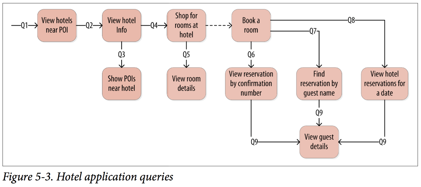
Hotel Data Model Sample

Let’s try the query-first approach to start designing the data model for our hotel application.

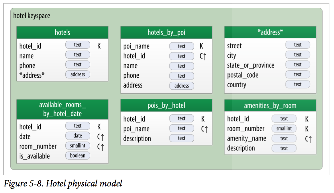
Hotel Keyspace

    CREATE KEYSPACE hotel
        WITH replication = {'class': 'SimpleStrategy', 'replication_factor' : 3};
    CREATE TYPE hotel.address (
        street text,
        city text,
        state_or_province text,
        postal_code text,
        country text
    );
    CREATE TABLE hotel.hotels_by_poi (
        poi_name text,
        hotel_id text,
        name text,
        phone text,
        address frozen<address>,
        PRIMARY KEY ((poi_name), hotel_id)
    ) WITH comment = 'Q1. Find hotels near given poi'
    AND CLUSTERING ORDER BY (hotel_id ASC) ;
    CREATE TABLE hotel.hotels (
        id text PRIMARY KEY,
        name text,
        phone text,
        address frozen<address>,
        pois set<text>
    ) WITH comment = 'Q2. Find information about a hotel';
    CREATE TABLE hotel.pois_by_hotel (
        poi_name text,
        hotel_id text,
        description text,
        PRIMARY KEY ((hotel_id), poi_name)
    ) WITH comment = 'Q3. Find pois near a hotel';

    CREATE TABLE hotel.available_rooms_by_hotel_date (
        hotel_id text,
        date date,
        room_number smallint,
        is_available boolean,
        PRIMARY KEY ((hotel_id), date, room_number)
    ) WITH comment = 'Q4. Find available rooms by hotel / date';
    CREATE TABLE hotel.amenities_by_room (
        hotel_id text,
        room_number smallint,
        amenity_name text,
        description text,
        PRIMARY KEY ((hotel_id, room_number), amenity_name)
    ) WITH comment = 'Q5. Find amenities for a room';

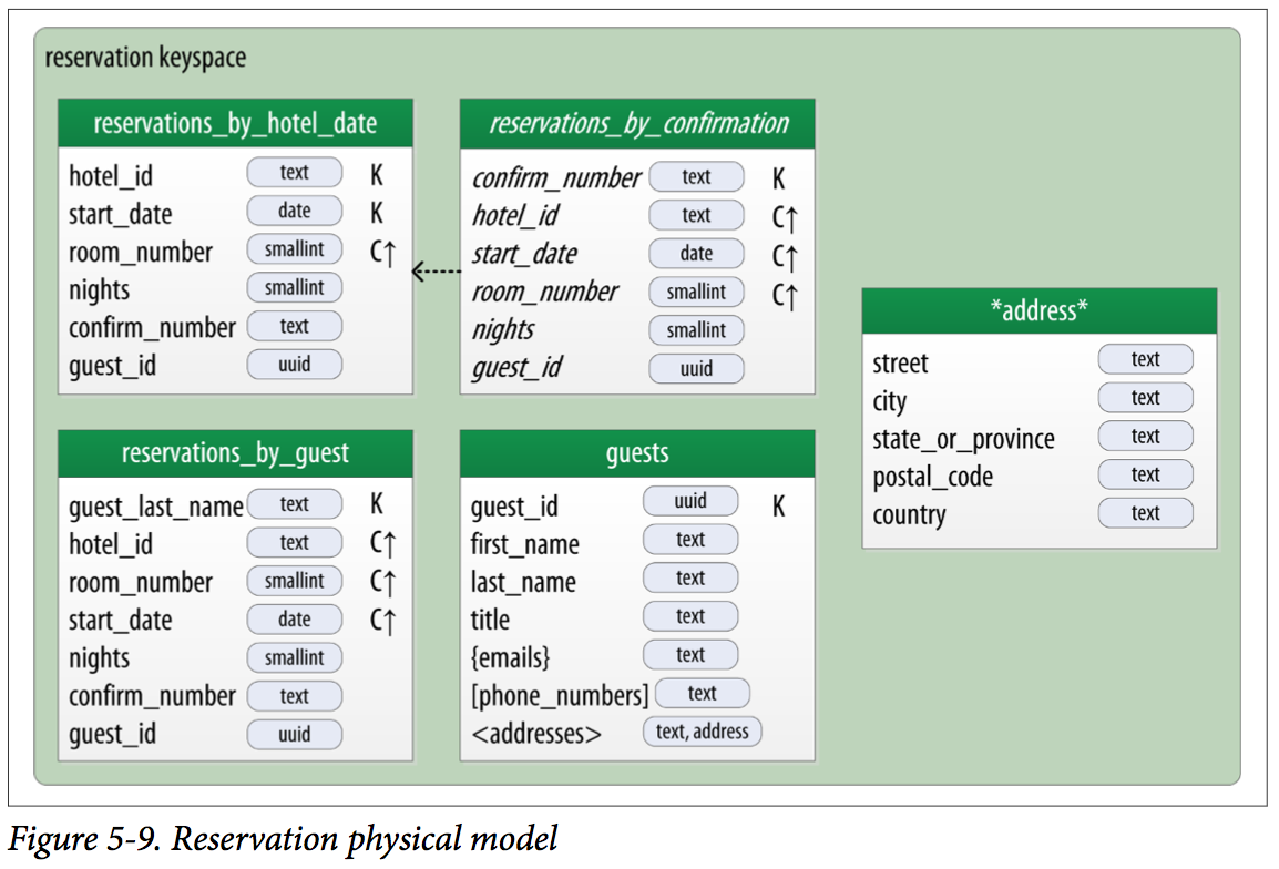
Reservation Keyspace

    CREATE KEYSPACE reservation
        WITH replication = {'class': 'SimpleStrategy', 'replication_factor' : 3};
    CREATE TYPE reservation.address (
        street text,
        city text,
        state_or_province text,
        postal_code text,
        country text
    );
    CREATE TABLE reservation.reservations_by_hotel_date (
        hotel_id text,
        start_date date,
        end_date date,
        room_number smallint,
        confirm_number text,
        guest_id uuid,
        PRIMARY KEY ((hotel_id, start_date), room_number)
    ) WITH comment = 'Q7. Find reservations by hotel and date';
    CREATE MATERIALIZED VIEW reservation.reservations_by_confirmation AS
        SELECT * FROM reservation.reservations_by_hotel_date
        WHERE confirm_number IS NOT NULL and hotel_id IS NOT NULL and
       start_date IS NOT NULL and room_number IS NOT NULL
        PRIMARY KEY (confirm_number, hotel_id, start_date, room_number);
    CREATE TABLE reservation.reservations_by_guest (
        guest_last_name text,
        hotel_id text,
        start_date date,
        end_date date,
        room_number smallint,
        confirm_number text,
        guest_id uuid,
        PRIMARY KEY ((guest_last_name), hotel_id)
    ) WITH comment = 'Q8. Find reservations by guest name';
    CREATE TABLE reservation.guests (
        guest_id uuid PRIMARY KEY,
        first_name text,
        last_name text,
        title text,
        emails set<text>,
        phone_numbers list<text>,
        addresses map<text, frozen<address>>,
        confirm_number text
    ) WITH comment = 'Q9. Find guest by ID';				

Cassandra Architecture

• Gossip and Failure Detection

  To support decentralization and partition tolerance, Cassandra uses a gossip protocol that allows each node to keep track of state information about the other nodes in the cluster. The gossiper runs every second on a timer.

  Because Cassandra gossip is used for failure detection, the Gossiper class maintains a list of nodes that are alive and dead.

  Here is how the gossiper works:

  1. Once per second, the gossiper will choose a random node in the cluster and initialize a gossip session with it. Each round of gossip requires three messages.

  2. The gossip initiator sends its chosen friend a GossipDigestSynMessage.

  3. When the friend receives this message, it returns a GossipDigestAckMessage.

  4. When the initiator receives the ack message from the friend, it sends the friend a GossipDigestAck2Message to complete the round of gossip.

• Snitches

  The job of a snitch is to determine relative host proximity for each node in a cluster, which is used to determine which nodes to read and write from. Snitches gather information about your network topology so that Cassandra can efficiently route requests. The snitch will figure out where nodes are in relation to other nodes.

• Rings and Tokens

  Data is assigned to nodes by using a hash function to calculate a token for the partition key. This partition key token is compared to the token values for the various nodes to identify the range, and therefore the node, that owns the data.

• Virtual Nodes

  Instead of assigning a single token to a node, the token range is broken up into multiple smaller ranges. Each physical node is then assigned multiple tokens (256 tokens by default).

  Vnodes make it easier to maintain a cluster containing heterogeneous machines. You can increase the num_tokens for more computing resources; also speed up some heavy-weight operations such as bootstrapping a new node, decommissioning a node, or repairing a node. This is because the load associated with operations on the multiple smaller ranges is spread more evenly across the nodes in the cluster.

• Partitioner

  Each row has a partition key that is used to identify the partition. A partitioner, then, is a hash function for computing the token of a partition key.

• Consistency Level

  For read queries, the consistency level specifies how many replica nodes must respond to a read request before returning the data. For write operations, the consistency level specifies how many replica nodes must respond for the write to be reported as successful to the client. Because Cassandra is eventually consistent, updates to other replica nodes may continue in the background.

  For both reads and writes, the consistency levels of ANY, ONE, TWO, and THREE are considered weak, whereas QUORUM and ALL are considered strong.

Memtables, SSTables, and Commit Logs

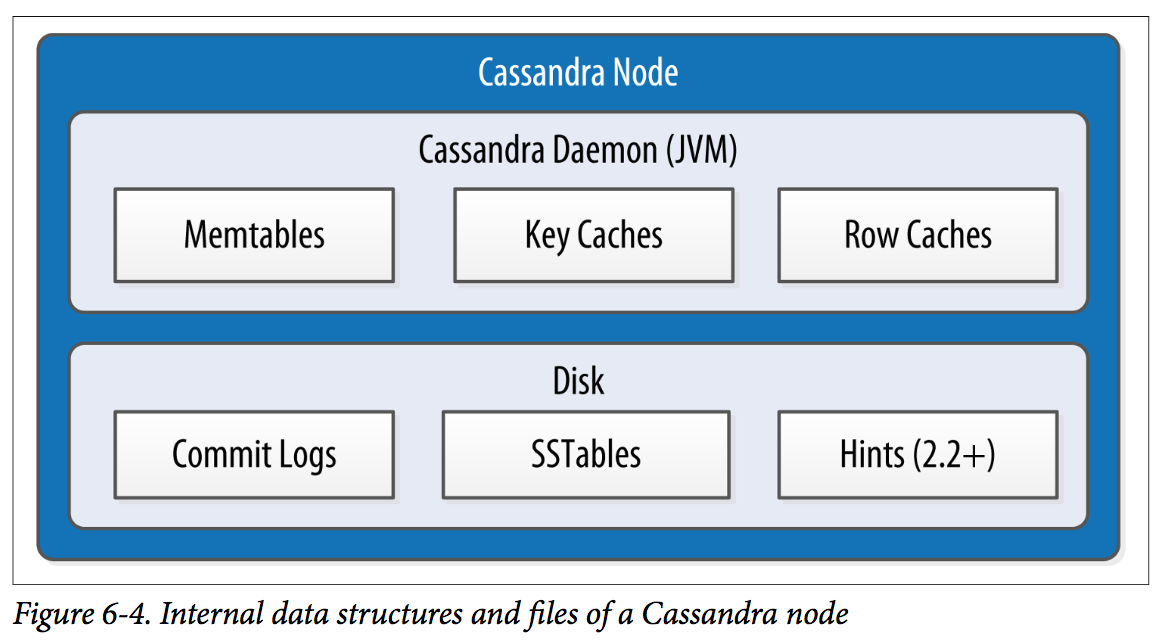
Cassandra stores data both in memory and on disk to provide both high performance and durability.

When you perform a write operation, it’s immediately written to a commit log. If you shut down the database or it crashes unexpectedly, the commit log can ensure that data is not lost. That’s because the next time you start the node, the commit log gets replayed.

After it’s written to the commit log, the value is written to a memory-resident data structure called the memtable. Each memtable contains data for a specific table. In early implementations of Cassandra, memtables were stored on the JVM heap, but improvements starting with the 2.1 release have moved the majority of memtable data to native memory. This makes Cassandra less susceptible to fluctuations in performance due to Java garbage collection.

When the number of objects stored in the memtable reaches a threshold, the contents of the memtable are flushed to disk in a file called an SSTable. A new memtable is then created. This flushing is a non-blocking operation; multiple memtables may exist for a single table, one current and the rest waiting to be flushed. They typically should not have to wait very long, as the node should flush them very quickly unless it is overloaded.

Each commit log maintains an internal bit flag to indicate whether it needs flushing. When a write operation is first received, it is written to the commit log and its bit flag is set to 1. There is only one bit flag per table, because only one commit log is ever being written to across the entire server. All writes to all tables will go into the same commit log, so the bit flag indicates whether a particular commit log contains anything that hasn’t been flushed for a particular table. Once the memtable has been properly flushed to disk, the corresponding commit log’s bit flag is set to 0, indicating that the commit log no longer has to maintain that data for durability purposes. Like regular logfiles, commit logs have a configurable rollover threshold, and once this file size threshold is reached, the log will roll over, carrying with it any extant dirty bit flags.

The SSTable is a concept borrowed from Google’s Bigtable. Once a memtable is flushed to disk as an SSTable, it is immutable and cannot be changed by the application. Despite the fact that SSTables are compacted, this compaction changes only their on-disk representation; it essentially performs the “merge” step of a mergesort into new files and removes the old files on success. Bloom filter is checked first before accessing disk. Because false-negatives are not possible, if the filter indicates that the element does not exist in the set, it certainly doesn’t; but if the filter thinks that the element is in the set, the disk is accessed to make sure.

Cache

• The key cache stores a map of partition keys to row index entries, facilitating faster read access into SSTables stored on disk. The key cache is stored on the JVM heap.

• The row cache caches entire rows and can greatly speed up read access for frequently accessed rows, at the cost of more memory usage. The row cache is stored in off-heap memory.

• The counter cache was added in the 2.1 release to improve counter performance by reducing lock contention for the most frequently accessed counters.

Compaction

As we already discussed, SSTables are immutable, which helps Cassandra achieve such high write speeds. However, periodic compaction of these SSTables is important in order to support fast read performance and clean out stale data values. A compaction operation in Cassandra is performed in order to merge SSTables. During compaction, the data in SSTables is merged: the keys are merged, columns are combined, tombstones are discarded, and a new index is created.

Hinted Handoff

This allows Cassandra to be always available for writes, and generally enables a cluster to sustain the same write load even when some of the nodes are down. It also reduces the time that a failed node will be inconsistent after it does come back online.

There is a practical problem with hinted handoffs (and guaranteed delivery approaches, for that matter): if a node is offline for some time, the hints can build up considerably on other nodes and causing flood requests to the back online node. To address this problem, Cassandra limits the storage of hints to a configurable time window. It is also possible to disable hinted handoff entirely.

Anti-Entropy, Repair, and Merkle Trees

Merkle tree is a data structure represented as a binary tree, and it’s useful because it summarizes in short form the data in a larger data set. In a hash tree, the leaves are the data blocks (typically files on a filesystem) to be summarized. Every parent node in the tree is a hash of its direct child node, which tightly compacts the summary.

In Cassandra, each table has its own Merkle tree; the tree is created as a snapshot during a major compaction, and is kept only as long as is required to send it to the neighboring nodes on the ring.

Staged Event-Driven Architecture (SEDA)

A stage is a basic unit of work, and a single operation may internally state-transition from one stage to the next. Because each stage can be handled by a different thread pool, Cassandra experiences a massive performance improvement. This design also means that Cassandra is better able to manage its own resources internally because different operations might require disk I/O, or they might be CPU-bound, or they might be network operations, and so on, so the pools can manage their work accord‐ ing to the availability of these resources.

A stage consists of an incoming event queue, an event handler, and an associated thread pool. Stages are managed by a controller that determines scheduling and thread allocation; Cassandra implements this kind of concurrency model using the thread pool java.util.concurrent.ExecutorService.

• Read (local reads) • Mutation (local writes) • Gossip • Request/response (interactions with other nodes) • Anti-entropy (nodetool repair) • Read repair • Migration (making schema changes) • Hinted handoff

Reference Resources

• Facebook RocksDB