Data-Intensive Applications

We call an application data-intensive if data is its primary challenge - the quantity of data, the complexity of data, or the speed at which it is changing.

The tools and technologies that help data-intensive applications store and process data have been rapidly adapting to these changes. New types of database systems (“NoSQL”) have been getting lots of attention, but message queues, caches, search indexes, frameworks for batch and stream processing, and related technologies are very important too.

As software engineers and architects, we need to have a technically accurate and precise understanding of the various technologies and their trade-offs if we want to build good applications. For that understandings, we have to dig deeper than buzzwords, grasp those enduring principles behind the rapid changes in technology.

C01 Foundations of Data Systems

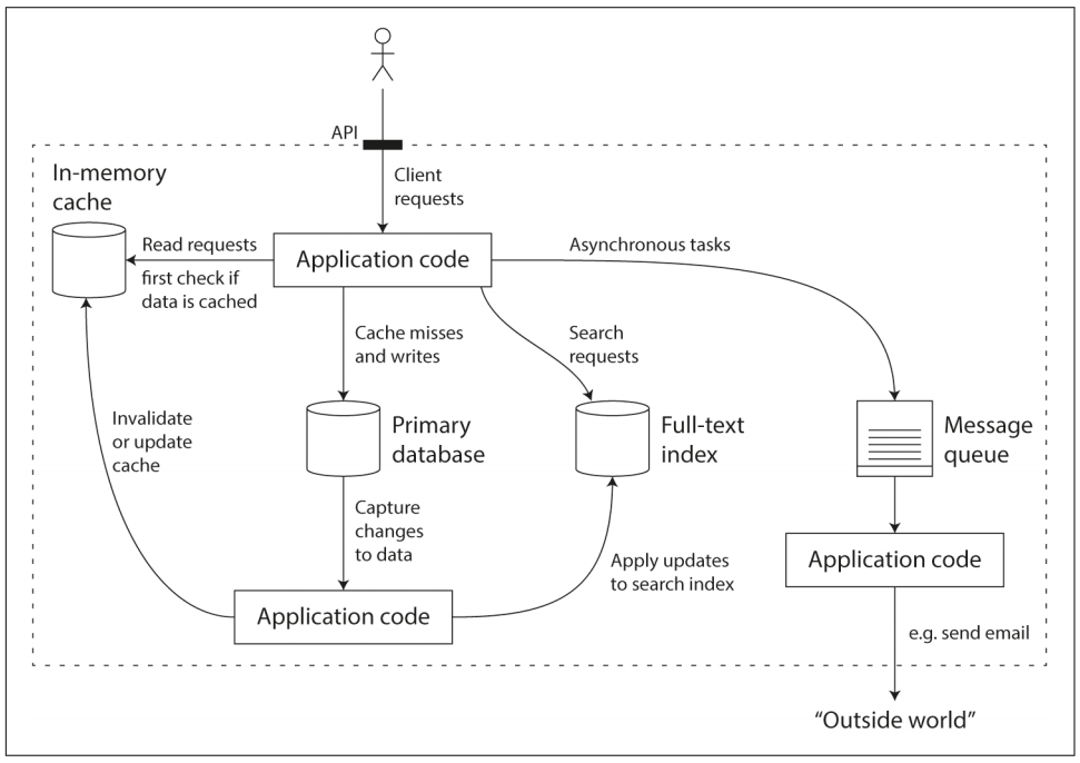
A data-intensive application is typically built from standard building blocks that provide commonly need functionality:

• Store data so that they, or another application can find it again later (databases).
• Remember the result of an expensive operation, to speed up reads (caches).
• Allow users to search data by keyword or filter it in various ways (search indexes).
• Send a message to another process, to be handled asynchronously (stream processing).
• Periodically crunch a large amount of accumulated data (bath processing).

We focus on three concerns that are important in most software systems: Reliability, Scalability and Maintainability.

Describe Performance

An SLA may state that the service is considered to be up if it has a median response time of less than 200ms and a 99th percentile under 1s (if the response time is longer, it might as well be down), and the service may be required to be up at least 99.9% of the time.

The median response time is 200ms, that means half your requests return in less than 200ms, half your requests take longer than that. The median is also known as the 50th percentile, abbreviated as p50.

An architecture that scales well for a particular application is built around assumptions of which operations will be common and which will be rare - the load parameters.

C02 Data Models and Query Languages

Later versions of the SQL standard added support for structured datatypes and XML data; this allowed multi-valued data to be stored within a single row, with support for querying and indexing inside those documents. These features are supported to varying degrees by Oracle, IBM DB2, MS SQL Server and PostgresSQL. A JSON datatype is also supported by several databases, including IBM DB2, MySQL, and PostgreSQL.

The driving forces behind the adoption of NoSQL (Not Only SQL) includes: A need for greater scalability (very large datasets or very high write throughput); A widespread preference for free and open source software; Specialized query operations that are not well supported by rational model; A desire for a more flexible schema, dynamic and expressive data models.

In a relational databases, the query optimizer automatically decides which parts of the query to execute in which order, and which indexes to use. You can just declare a new index without having to change your queries, and have optimizer to take advantage of the new index.

The main arguments in favor of the document data model are schema flexibility, better performance due to locality, and sometimes it is closer to the data structures. It’s schema-on-read (the structure of the data is implicit, and only interpreted when the data is read), similar to dynamic (runtime) type checking in programming languages.

MapReduce Querying

MapReduce is a programming model for processing large amounts of data in bulk across many machines. The logic of the query is expressed with snippets of code, which are called repeated by the processing framework. It is based on the map (also know as collect) and reduce (also known as fold or inject) functions that exist in many functional programming languages.

The sample of MongoDB’s MapReduce feature as follows:

db.observations.mapReduce(
  function map() {
    var year = this.observationTimestamp.getFullYear();
    var month = this.observationTimestamp.getMonth() + 1;
    emit(year + "-" + month, this.numAnimals);
  },
  function reduce(key, values) {
    return Array.sum(values);
  },
  {
    query: { family: "Sharks" },
    out: "monthlySharkReport"
  }
);

C03 Storage and Retrieval

In order to efficiently find the value for a particular key in the database, we need a different data structure: an index. But any kind of index usually slows down writes, because the index also needs to be updated every time data is written.

Hash Indexes

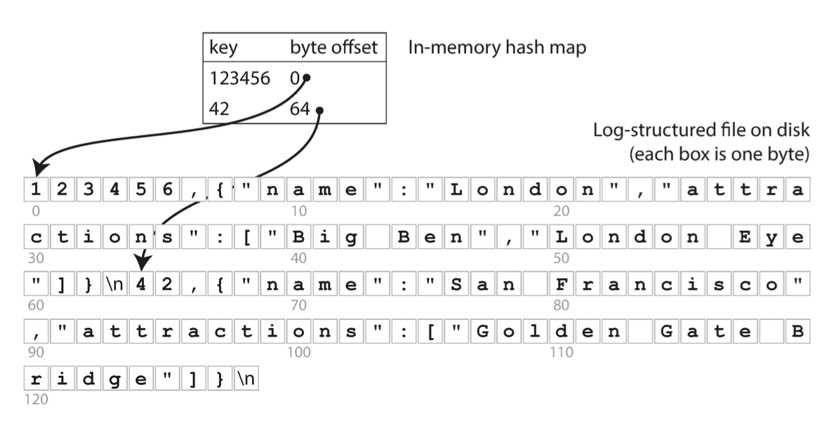
• Storing a log of key-value pairs in a CSV-like format consists only of appending to the file, indexed with an in-memory hash map. It’s faster and simpler to use a binary format that first encodes the length of a string in bytes, followed by the raw string (without need for escaping).
• To avoid running out of disk space, A good solution is go break the log into segments of a certain size by closing a segment file when it reaches a certain size, and making subsequent writes to a new segment file. We can run a dedicated thread to perform compaction and segment merging simultaneously.
• Deleting a key and its associated value, you have to append a special deletion record to the data file (sometimes called a tombstone). The merging process will discard any previous values during merge.
• Concurrency control, as writes are appended to the log in a strictly sequential order, a common implementation choice is to have only one write thread, or shard the log and synchronization is done via a per-shard mutex.

However, the hash table index must fit in memory and range queries are not efficient.

SSTables and LSM-Trees

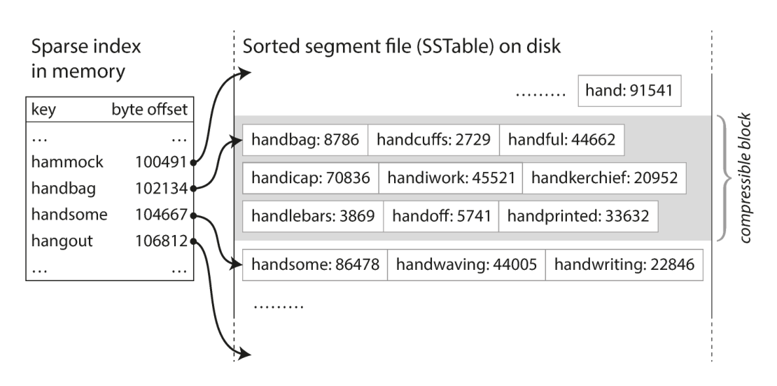
• Sorted String Table (SSTable) requires that the sequence of key-value pairs is sorted by key. Use mergesort algorithm to produces a new merged segment file, also sorted by key. You just need a set of sparse index in memory to align with a list of segment file. When multiple segments contain the same key, we can keep the value from the most recent segment and discard the values in older segments.
• In order to find a particular key in the file, you just need to keep a sparse index in memory, one key for every few kilobytes of segment file is sufficient. Since read requests need to scan over several key-value pairs in the requested range anyway, it is possible to group those records into a block and compress it before writing to disk.
• Use an in-memory balanced tree data structure (red-black trees or AVL trees), sometimes called memtable, you can insert keys in any order and read them back in sorted order. When the memtable gets bigger than some threshold (typically a few megabytes), write it out to disk as an SSTable file. In order to serve a read request, first try to find the key in the memtable, then in the most recent on-disk segment, then in the next-older segment, etc. From time to time, run a merging and compaction process in the background to combine segment files and to discard overwritten or deleted values.
• In order to avoid crash problem, we can keep a separate log on disk to which every write is immediately appended. This log is not in sorted order, because its only purpose is to restore the memtable after a crash. Every time the memtable is written out to an SSTable, the corresponding log can be discarded.
• Making an LSM-tree out of SSTable. Log-Structured Merge-Tree (LSM-Tree), building on log-structured filesystems. Such as Lucene, an indexing engine for full-text search used by Elasticsearch and Solr, uses a similar method for storing its term dictionary. This is implemented with a key-value structure where the key is a word (a term) and the value if the list of IDs of all the documents that contain the word.
• LSM-tree algorithm can be slow when looking up keys that don’t exist in database: you have to check the memetable, then the segments all the way back to the oldest (possibly having to read from disk for each one), You can use additional Bloom filters to optimize this kind of access.
• There are also different strategies to determine the order and timeing of how SSTables are compacted and merged. The most common options are size-tiered compaction (newer and smaller SSTables are successively merged into older and larger SSTables); leveled compaction (The key range is split up into smaller SSTables and older data is moved into separate levels).
• Full-text search and fuzzy indexes. In LevelDB, this in-memory index is a sparse collection of some of the keys, but in Lucene, the in-memory index is a finite state automation over the characters in the keys, similar to a trie. which supports efficient search for words within a given edit distance.

B-Trees

• The B-trees break the database down into fixed-size blocks or pages. Traditionally 4KB in size, and read or write one page at a time. Each page can be identified using an address or location, which allows one page to refer to another, and finally construct a tree of pages.
• This algorithm ensures that the tree remains balanced: a B-tree with n keys always has a depth of O(logn). A four-level tree of 4KB pages with a branching factor of 500 can store up to 256TB.

Multi-column Indexes

To support two-dimensional range query. One option is to translate a two-dimensional location into a single number using a space-filling curve, and then to use a regular B-tree index. More commonly, specialized spatial indexes such as R-trees are used.

The performance advantage of in-memory databases is not due to the fact that they don’t need to read from disk, but because they can avoid the overheads of encoding in-memory data structure in a form that can be written to disk. And also in-memory database provides more flexible data models.

C04 Encoding and Evolution

Binary schema-driven formats like Thrift, Protocol Buffers and Avro allow compact, efficient encoding with clearly defined forward and backward compatibility semantics. The schemas can be useful for documentation and code generation in statically typed languages.

Apache Avro

Our example schema, written in Avro IDL, might look like this:

record Person {
    string               userName;
    union { null, long } favoriteNumber = null;
    array<string>        interests;
}

The equivalent JSON representation of that schema is:

{
    "type": "record",
    "name": "Person",
    "fields": [
        {"name": "userName",       "type": "string"},
        {"name": "favoriteNumber", "type": ["null", "long"], "default": null},
        {"name": "interests",      "type": {"type": "array", "items": "string"}}
    ]
}

Looking at the following example data record encoded using Avro. To parse the binary data, you go through the fields in the order that they appear in the schema and use the schema to tell you the data type of each fields.

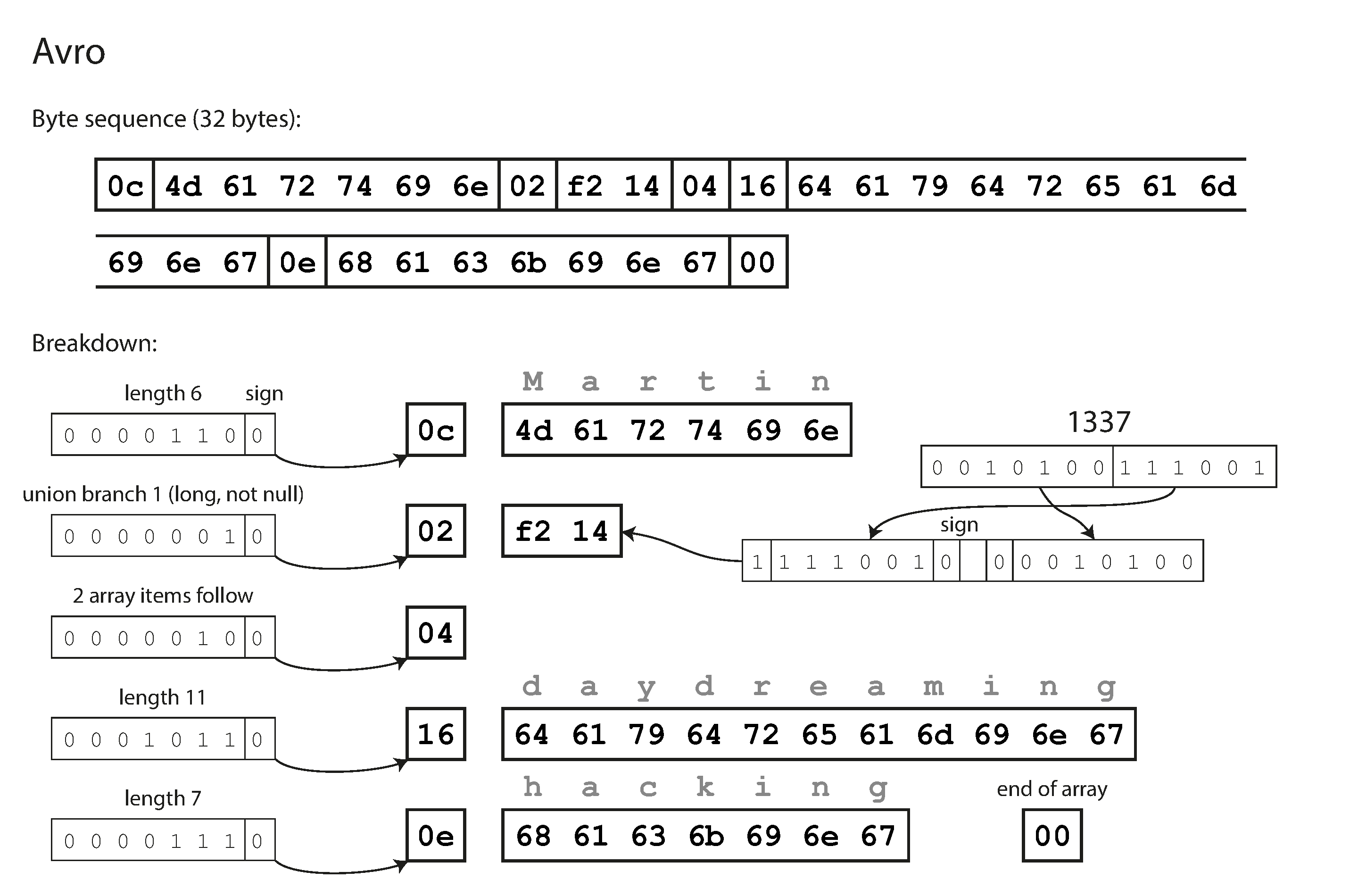
The key idea with Avro is that the writer’s schema and the reader’s schema don’t have to be the same–they only need to be compatible. When data is decoded (read), the Avro library resolves the differences by looking at the writer’s schema and the reader’s schema side by side and translating the data from the writer’s schema into the reader’s schema.

C05 Replication

Concurrent Writes Resolution

To capture causal dependencies between two clients concurrently editing a shopping cart. The server maintains a version number for every key, increments the version number every time that key is written, and stores the new version number along with the value written. The value should be a map with each client (id) and their merged changes.

When a client writes a key, it must include the version number from the prior read, and it must merge together all values that it received in the prior read.

This algorithm ensures that no data is silently dropped, but the clients have to clean up afterward by merging the concurrently written values, which is called Merge Siblings.

With multiple replica, we need to use a version number per replica as well as per key.

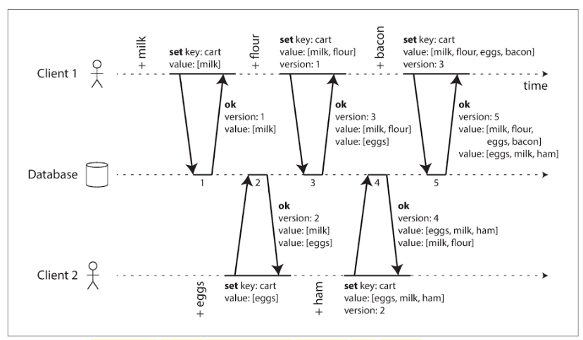
Please note the step 4: client2 received the two values [milk] and [eggs] from the server in the last response (version:2), so client2 now merges those values and adds ham to form a new value [eggs, milk, ham]. It sends that value to the server, along with the previous version number 2. The server detects that version 2 overwrites [eggs] but is concurrent with [milk, flour] which is version 3. so return all values with version 4.

C06 Partitioning

The goal of partitioning is to spread the data and query load evenly across multiple machines, avoid hot spots (nodes with disproportionately high load). This requires choosing a partitioning schema that is appropriated to your data, and rebalancing the partitions when nodes are added to or removed from the cluster.

We have two main approaches to partitioning:

Key Range Partitioning

Where keys are sorted, and a partition owns all the keys from some minimum up to some maximum. Sorting has the advantage that efficient range queries are possible, but there is a risk of hot spots if the application often access keys that are close together in the sorted order.

In this approach, partitions are typically rebalanced dynamically by splitting the range into two subranges when a partition gets too big.

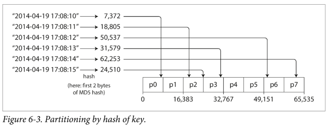
Hash Partitioning

Where a hash function is applied to each key, and a partition owns a range of hashes. This method destroys the ordering of keys, making range queries inefficient, but may distribute load more evenly. (The MD5 hash function generates 128 bits, which gives 32 characters if encode it as hexadecimal). The following chart uses the first 2 bytes of MD5 hash, which covers a total of 2^16 = 65536 partitions.

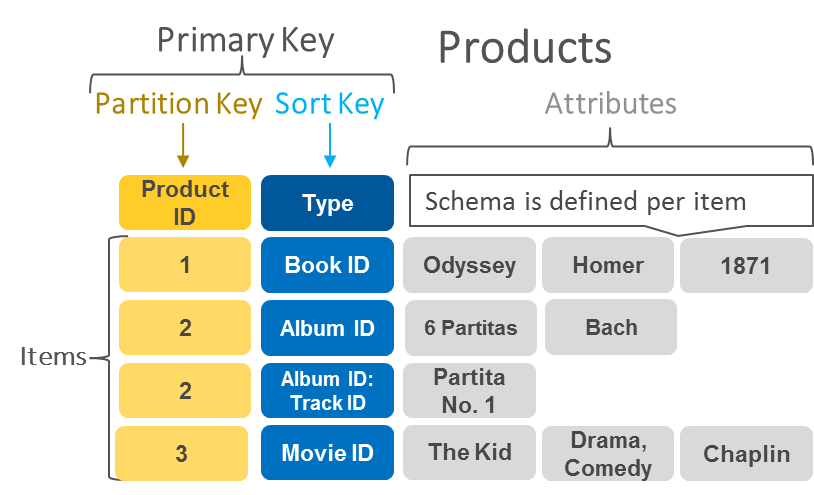
Compound Primary Key

To achieve a compromise between above two partition strategies. A table in Cassandra can be declared with a compound primary key consisting of several columns. Only the first part of that key is hashed to determine determine the partition, but the other columns are used as concatenated index for sorting the data in SSTables. If it specifies a fixed value for the first column, it can perform an efficient range scan over the other columns of the key.

The concatenated index approach enables an elegant data model for one-to-many relationships. For example, on a social media site, one user may post many updates. If the primary key for update is chosen to be (user_id, update_timestamp), then you can efficiently retrieve all updates made by a particular user within some time interval, sorted by timestamp. Different users may be stored on different partitions, but within each user, the updates are stored ordered by timestamp on a single partition.

As below chart shows, the primary key consists of partition key and sort key.

Skewed Workloads and Relieving Hot Spots

In the extreme case where all reads and writes are for the same key, you still end up with all requests being routed to the same partition. For example, on a social media site, a celebrity user with millions of followers may cause a storm of activity when they do something. The even can result in a large volume of writes to the same key.

Today, most data systems are not able to automatically compensate for such a highly skewed workload, so it’s the responsibility of the application to reduce the skew. For example, if one is known to be very hot, a simple technique is to add a random number to the beginning or end of the key, allowing those keys to be distributed to different partitions.

However, you need some way of keeping track of which keys are being split. Any reads now have to do additional work, as they have to read the data from all sub keys and combine it.

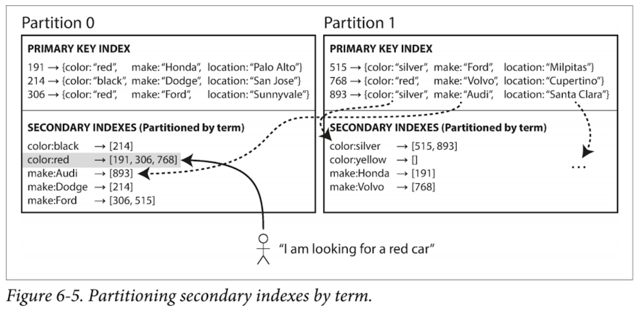
Partitioning Secondary Indexes

A secondary index also needs to be partitioned, and there are two methods:

• Document-partitioned indexes (local indexes), where the secondary indexes are stored in the same partition as the primary key and value. This means that only a single partition needs to updated on write, but a read of the secondary index requires a scatter/gather across all partitions.
• Term-partitioned indexes (global indexes), where the secondary indexes are partitioned separately, using the indexes values. An entry in the secondary index may include records from all partitions of the primary key. When a document is written, several partitions of the secondary index need to be updated; however, a read can be served from a single partitions

Strategies for Rebalancing

When partitioning by the hash of a key, it’s best to divide the possible hashes into ranges and assign each range to a partition. but do NOT use mod N approach, because if the number of nodes N changes, most of the keys will need to be moved from one node to another. Such frequent moves make rebalancing excessively expensive.

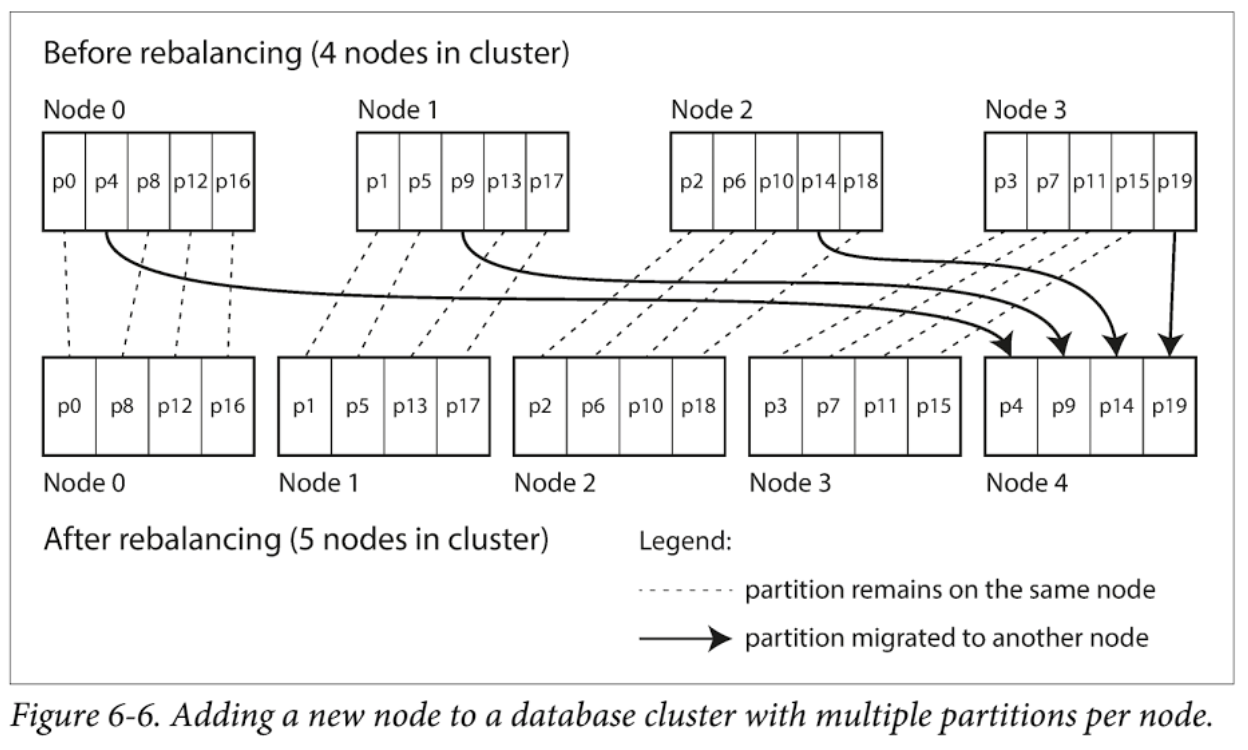
We need an approach that doesn’t move data around more that necessary, Fixed number of partitions: create many more partitions than there are nodes, and assign several partitions to each node. For example, a database running on a cluster of 10 nodes may be split into 1,000 partitions for the outset so that approximately 100 partitions are assigned to each node.

Now, if a node is added to the cluster, the new node can steal a few partitions from every existing node until partitions are fairly distributed once again. The key range partitioned databases such as HBase and RethinkDB create partitions dynamically. When a partition grows to exceed a configured size (10GB), it is split into two partitions.

Request Routing

There are three different ways of routing a request to the right node. (service discovery).

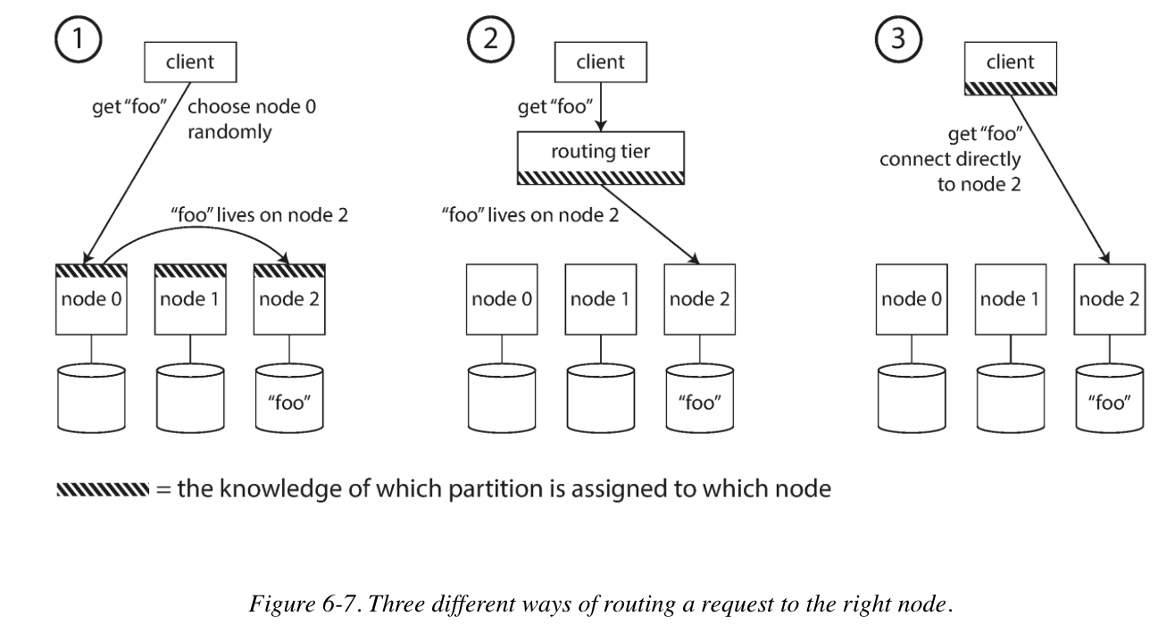
Many distributed data systems rely on a separate coordination service such as ZooKeeper to keep track of this cluster metadata. Each node register itself in ZooKeeper, and ZooKeeper maintains the authoritative mapping of partitions to nodes. Other actors, such as the routing tier or the partitioning-aware client, can subscribe to this information in ZooKeeper. Whenever a partition changes ownership, or a node is added or removed, ZooKeeper notifies the routing tier so that it can keep its routing information up to date.

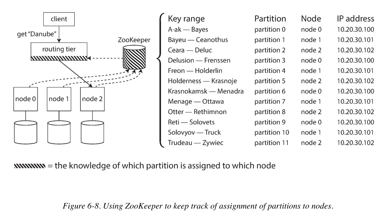
Key -> MD5(Key) -> First 2 Bytes -> Lookup Partition ID -> Get Node ID -> Get IP Address

C07 Transactions

The Meaning of ACID

• Atomicity: The ability to abort a transaction on error and have all writes from that transaction discarded is the defining feature of ACID atomicity.
• Consistency: The idea of consistency is that you have certain statements about your data (invariants) that must always be true. However it’s the application’s responsibility to preserve consistency, not something that the database can guarantee.
• Isolation: Means that concurrently executing transactions are isolated from each other: they cannot step on each other’s toes.
• Durability: Once a transaction has committed successfully, any data it has written will not be forgotten, even if there is a hardware fault or the database crashes.

Single-object writes

For example, imagine you are writing a 20KB JSON document to a database. The storage engines almost universally aim to provide atomicity and isolation on the level of a single object. Atomicity can be implemented using a log for crash recovery, and isolation can be implemented using a lock on each object.

Weak Isolation Levels

Databases have long tried to hide concurrency issues from providing transaction isolation:

• Serializable isolation, which has a performance cost.
• Weak (non-serializable) isolation, which protect against some concurrency issues, but not all.

Read Committed

The most basic level of transaction isolation is read committed. It makes two guarantees:

1. When reading from the database, you will only see data that has been committed (no dirty read). To prevent dirty reads, for every object that is written, the database remembers both the old committed value and the new value set by the transaction that currently holds the write lock. While the transaction is ongoing, any other transactions that read the object are simply given the old value. Only when the new value is committed do transactions switch over to reading the new value.

2. When writing to the database, you will only overwrite data that has been committed (no dirty writes). Mostly databases prevent dirty writes by using row-level locks: when a transaction wants to modify a particular object, it must first acquire a lock on that object and hold that lock until the transaction is committed or aborted.

Snapshot Isolation

With above read committed approach, there could be still some temporary inconsistency among the transaction. Which can not be tolerated in some situations: Backups or Analytic queries and integrity checks.

Snapshot isolation is the most common solution to this problem. The idea is that each transaction reads from a consistent snapshot of the database–that is, the transaction sees all the data that was committed in the database at the start of the transaction. Even if the data is subsequently changed by another transaction, each transaction sees only the old data from that particular point in time.

Like read committed isolation, implementations of snapshot isolation typically use write locks to prevent dirty writes. However, reads do not require any locks. A key principal of snapshot isolation is readers never block writes, and writes never block readers.

To implement snapshot isolation, the database must potentially keep several different committed versions of an object, because various in-progress transactions may need to see the state of the database at different points in time. Because it maintains several versions of an object side by side, this technique is known as multi-version concurrency control (MVCC).

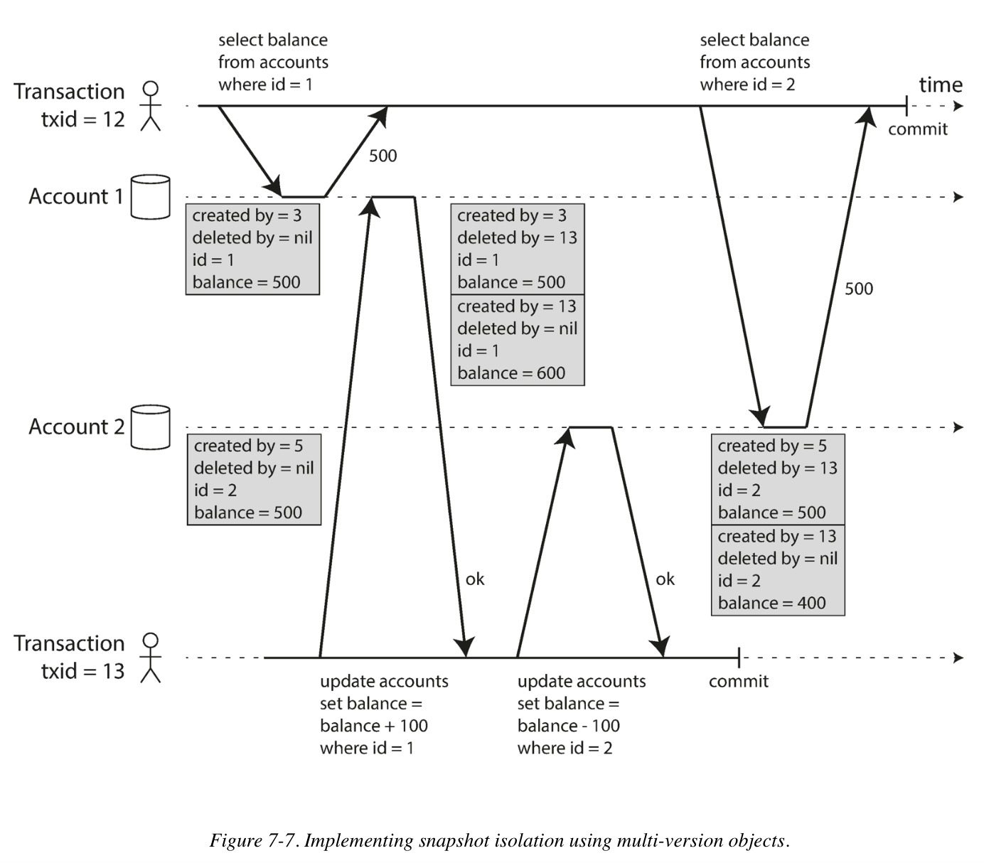
An update is internally translated into a delete and a create. At some later time, when it is certain that no transaction can any longer access the deleted data, a garbage collection process in the database removes any rows marked for deletion and frees their space.

Visibility rules for observing a consistent snapshot:

• At the time when the reader’s transaction started, the transaction that created the object had already committed.
• The object is not marked for deletion, or if it is, the transaction that requested deletion had not yet committed at the time when the reader’s transaction started.

How do indexes work in a MVCC database?

• One option is to have the index simply point to all versions of an object and require an index query to filter out any object versions that are not visible to the current transaction.
• Another approach is they use an append-only/copy-on-write variant that does not overwrite pages of the tree when they are updated, but instead creates a new copy of each modified page. So every write transaction creates a new B-tree root, later requires a background process for compaction and garbage collection.

Preventing Lost Updates

The read committed and snapshot isolation levels we’ve discussed so far have been primarily about the guarantees of what a read-only transaction can see in the presence of concurrent writes.

Also the lost update problem can occur if an application reads some value from the database, modifies it, and writes back the modified value (a read-modify-write cycle). If two transactions do this concurrently, one of the modifications can be lost. Such as incrementing a counter; making a local change to a complex value; two users editing a wiki page at the same time.

A variety of solutions have been developed:

• Atomic write operations

UPDATE counters SET value = value + 1 WHERE key = 'foo';

• Explicit locking

BEGIN TRANSACTION;

SELECT * FROM figures WHERE name = 'robot' AND game_id = 222 FOR UPDATE;

UPDATE figures SET position = 'c4' WHERE id = 1234;

COMMIT;

• Automatically detecting lost updates

Allow them to execute in parallel and, if the transaction manager detects a lost update, abort the transaction and force it to retry its read-modify-write cycle.

• Compare-and-set

UPDATE wiki_pages SET content = 'new content' WHERE id = 1234 AND content = 'old content';

Write Skew and Phantom Reads

Write Skew: A transaction reads something, makes a decision based on the value it saw, and writes the decision to the database. However, by the time the write is made, the premise of the decision is no longer true. Only serializable isolation prevents this anomaly.

Three different approaches to implementing serializable transactions:

• Literally executing transactions in a serial order
• Two-phase locking
  1. The blocking of readers and writers is implemented by having a lock on each object in the database. The lock can either be in shared mode or in exclusive mode.
  2. The first phase is when the locks are acquired, and the second phase is when all the locks are released.
• Serializable snapshot isolation (SSI)

Serializable Snapshot Isolation (SSI)

A fairly new algorithm that avoids most of the downsides of the previous approaches. It uses an optimistic approach, allowing transactions to proceed without blocking. When a transaction wants to commit, it is checked, and it is aborted if the execution was not serializable.

Optimistic concurrency control techniques tend to perform better than pessimistic ones if contention between transactions is not too high. And contention can be reduced with commutative atomic operations.

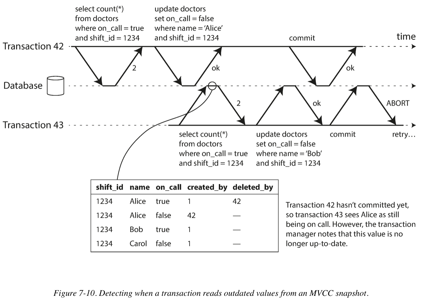
Decisions based on an outdated premise

• Detecting stale MVCC reads

The database needs to track when a transaction ignores another transaction’s writes due to MVCC visibility rules; When the transaction wants to commit, the database checks whether any of the ignored writes have now been committed. If so, the transaction must be aborted.

Also, why wait until committing? This can avoid unnecessary aborts, SSI preserves snapshot isolation’s support for long-running reads from a consistent snapshot.

• Detecting writes that affect prior reads

The second case to consider is when another transaction modifies data after it has been read.

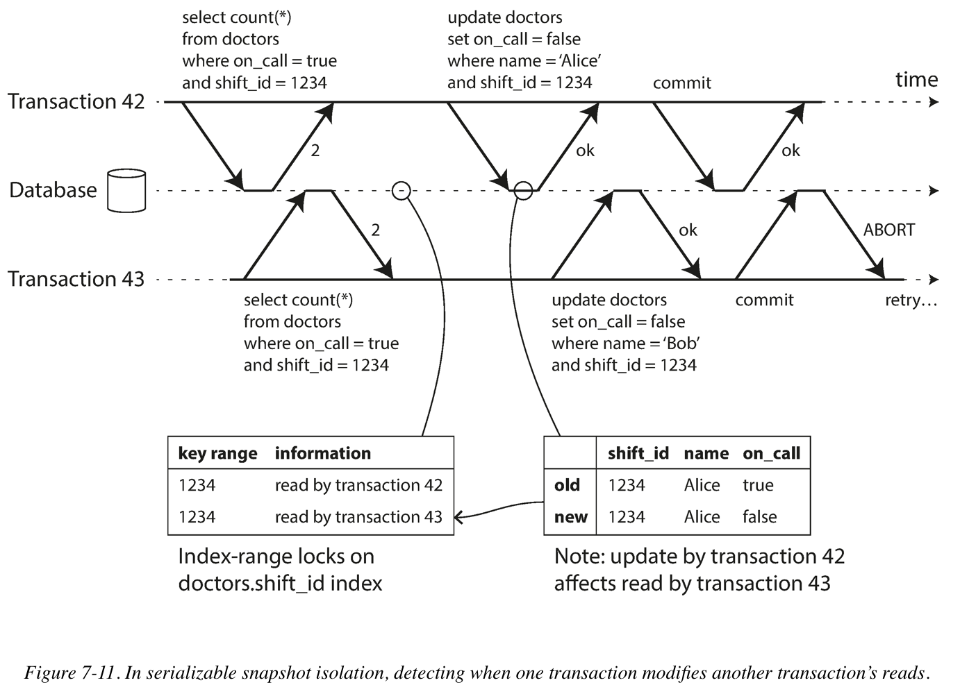
Compare to two-phase locking, the big advantage of serializable snapshot isolation is that one transaction doesn’t need to block waiting for locks held by another transaction. Like under snapshot isolation, writers don’t block readers, and vice versa. This design principal makes query latency much more predictable and less variable. In particular, read-only queries can run on a consistent snapshot without requiring any locks, which is very appealing for read-heavy workloads.

C08 The Trouble with Distributed System

Distributed systems are different from programs running on a single computer: there is no shared memory, only message passing via an unreliable network with variable delays, and the systems may suffer from partial failures, unreliable clocks, and processing pauses.

TCP Versus UDP

Some latency-sensitive application, such as videoconferencing and Voice over IP (VoIP), use UDP rather than TCP. It’s a trade-off between reliability and variability of delays: as UDP does not perform flow control and does not retransmit lost packages, it avoids some of the reasons for variable network delays.

Monotonic Versus Time-of-Day Clocks

A monotonic clock is suitable for measuring a duration (time interval), such as a timeout or a service’s response time. (System.nanoTime in Java). The are guaranteed to always move forward.

Time-of-day clocks are usually synchronized with NTP (limited by the network round-trip time). But if the local clock is too far ahead of the NTP server, it may be forcibly reset and appear to jump back or forward, make it unsuitable for measuring elapsed time.

Process Pauses

Let’s consider you have a database with a single leader per partition. Only the leader is allowed to accept writes. The leader needs to obtain a lease from the other nodes. Only one node can hold the lease at any one time, for some amount of time. In order to to remain leader, the node must periodically renew the lease before it expires. If the node fails, it stops renewing the lease, so another node can take over when it expires.

You can image the request-handling loop looking something like this:

while (true) {
  request = getIncomingRequest();

  // Ensure that the lease always has at least 10 seconds remaining
  if (lease.expiryTimeMillis - System.currentTimeMillis < 10000) {
    lease = lease.renew();
  }

  // Process could pause at this point:
  // A JVM GC to stop all running threads
  // A virtual machine can be suspended
  // End-user devices may also be suspended
  // OS context-switches to another thread, or hyper-switches to a different virtual machine
  // A thread may be paused waiting for a slow disk I/O operation to complete
  // OS may spend most of its time swapping pages in and out of memory
  // A Unix process can be paused by sending it the SIGSTOP signal

  if (lease.isValid()) {
    process(request);
  }
}

Limiting the impact of garbage collection

• Treat GC pauses like brief planned outages of a node. If the runtime can warn the application that a node soon requires a GC pause, the application can stop sending new requests to that node, wait for it to finish processing outstanding requests, and then perform the GC while no requests are in process.

• A variant of this idea is to use the garbage collector only for short-lived objects (which are fast to collect) and restart processes periodically.

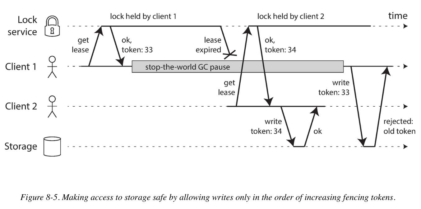
Fencing Tokens

When using a lock or lease to protect access to some resource, we need to ensure that a node that is under a false belief of being “the chosen one” cannot disrupt the rest of the system. A fairly simple technique is called fencing, every time the lock server grants a lock or lease, it also returns a fencing token.

If ZooKeeper is used as lock service, the transaction ID zxid or the node version cversion can be used as fencing token. For server resources that do not explicitly support fencing tokens, you can include the fencing token in the file name.

C09 Consistency and Consensus

Linearizability

Its goal is to make replicated data appear as though there were only a single copy, and to make all operations act on it atomically. Although linearizability is appealing because it is easy to understand (it makes a database behave like a variable in a single threaded program), it has the downside of being slow, especially in environments with large network delays.

Linearizability is useful in a few areas:

• Locking and leader election
• Constraints and uniqueness guarantees
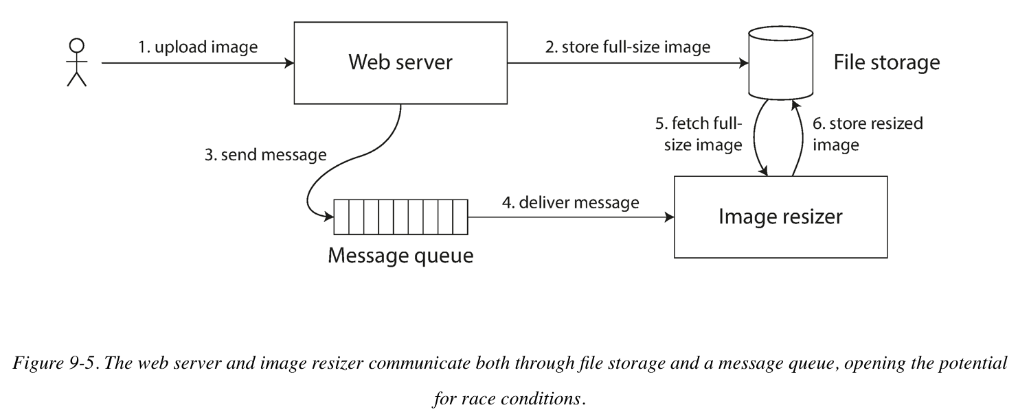
• Cross-channel timing dependencies (image resizer sample)

Ordering Guarantees

Unlike linearizability, which puts all operations in a single, totally ordered timeline, ordering and causality provides us with a weaker consistency model: some things can be concurrent, so the version history is like a timeline with branching and merging, so it is much less sensitive to network problems.

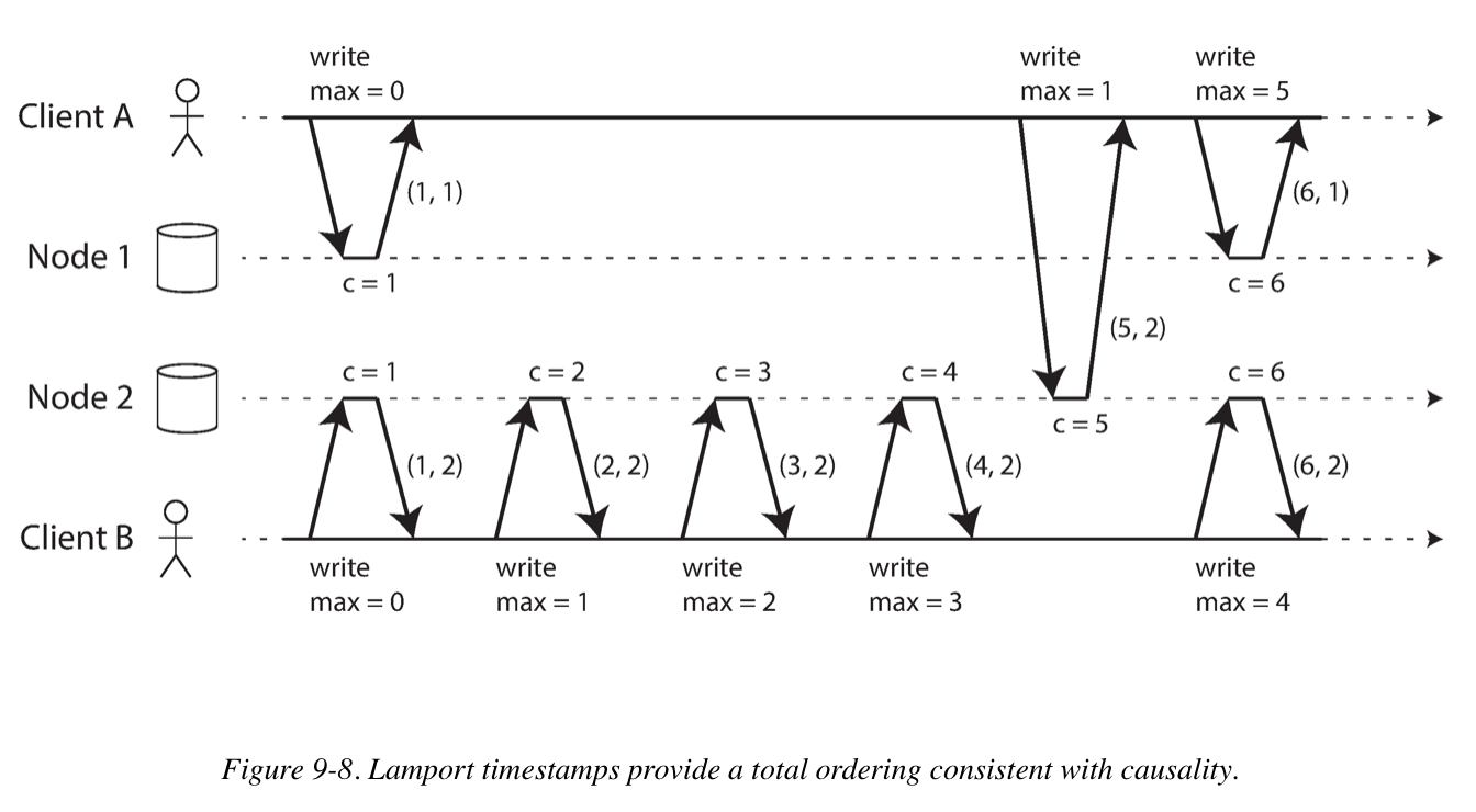
Lamport timestamps

In a database with single-leader replication, the leader can simply increment a counter for each operation in the replication log. Which is called sequence number ordering.

But with a multi-leader or leader-less database, or the database is partitioned. The key idea about Lamport timestamps, which makes them consistent with causality, is the following: every node and every client keeps track of the maximum counter value it has seen so far, and includes that maximum on every request. When a node receive a request or response with a maximum counter value greater than its own counter value, it immediately increases its own counter to that maximum.

The Lamport timestamp is then simply a pair of (counter, node ID).

Total Order Broadcast

Total order broadcast is usually described as a protocol for exchanging messages between nodes. It requires two safety properties: Reliable delivery (no lost) and Totally ordered delivery (in the same order).

Another way of looking at total order broadcast is that it is a way of creating a log (as in a replication log, transaction log, or write -ahead log): delivering a message is like appending to the log. Since all nodes must delivery the same messages in the same order, all nodes can read the log and see the same sequence of messages.

• Implementing linearizable storage using total order broadcast.

  You can implement a linearizable compare-and-set operation by using total order broadcast as an append-only log.

  1. Append a message to the log, tentatively indicating the username you want to claim.
  2. Read the log, and wait for the message you appended to be delivered back to you.
  3. Check for any messages claiming the username that you want. If the first message for your desired username is your own message, then you are successful.

• Implementing total order broadcast using linearizable storage

The easiest way is to assume you have a linearizable register that stores an integer and that has an atomic increment-and-get operation. For every message you want to send through total order broadcast, you increment-and-get the linearizable integer, and then attach the value you got from the register as a sequence number to the message.

Atomic Commit and Two-Phase Commit (2PC)

Two-phase commit is an algorithm for achieving atomic transaction commit across multiple nodes.

A 2PC transaction begins with the application reading and writing data on multiple database nodes (also called participants). When the application is ready to commit, the coordinator begins phase 1: it sends a prepare request to each of the nodes, asking them whether they are able to commit. The coordinator then tracks the responses from the participants and decides to send out a commit or abort request.

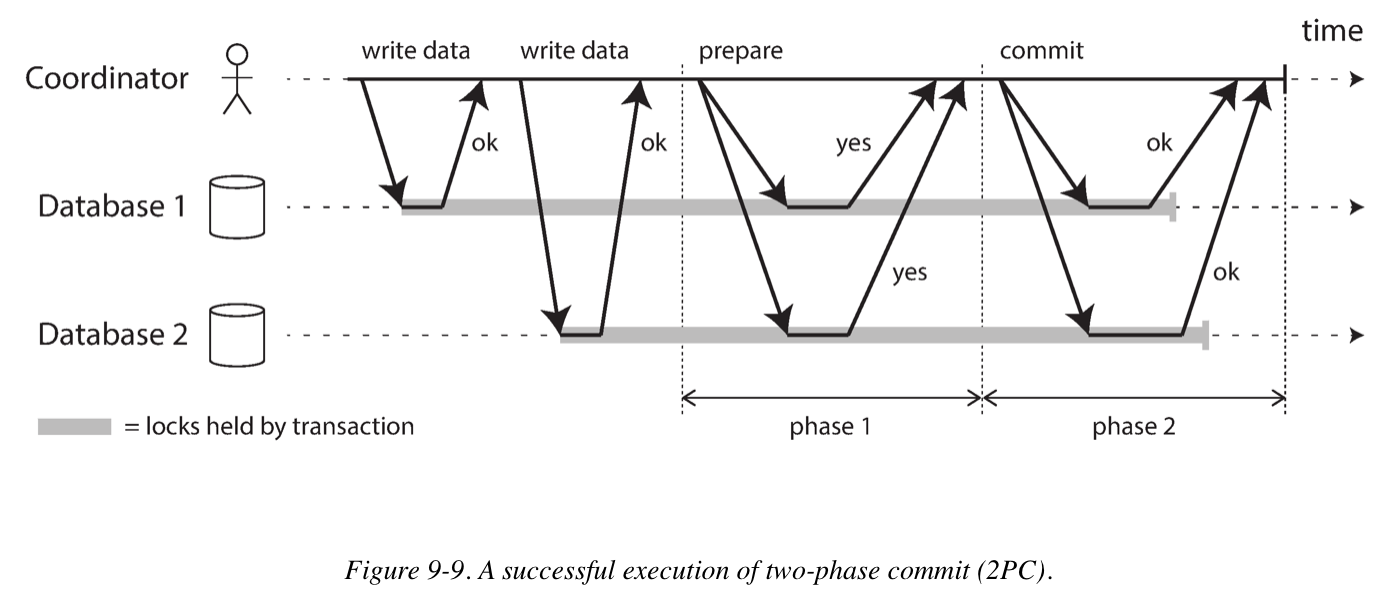
To understand why it works, let’s break down the process:

1. When the application wants to begin a distribution transaction, it requests a transaction ID from the coordinator, or provided by the application. This transaction ID must be globally unique.

2. The application begins a single-node transaction on each of the participants, or replicated by a single-leader, and attaches the global unique transaction ID to the participants. If anything went wrong, the coordinator or any of the participants can abort.

3. When the application is ready to commit, the coordinator sends a prepare request to all participants, tagged with the global transaction ID. If any of these request fails or times out, the coordinator sends an abort request.

4. When a participant receive the prepare request, it makes sure that it can definitely commit the transaction under all circumstances. By replying “yes” to the coordinator, the node promises to commit the transaction without error if requested.

5. When the coordinator has received responses to all prepare requests, it makes a definitive decision on whether to commit or abort the transaction. The coordinator must write the decision to its transaction log on disk in case it subsequently crashes.

6. Once the coordinator’s decision has been written to disk, the commit or abort request is sent to all participants. If this request fails or times out, the coordinator must retry forever until it succeeds.

Much of the performance cost inherent in two-phase commit is due to the additional disk forcing (fsync) that is required for crash recovery, and the additional network round-trips.

XA Transactions

X/Open XA (short for Extended Architecture) is a standard for implementing two-phase commit across heterogeneous technologies, has been widely supported by many traditional relational database. XA assumes that your application uses a network driver or client library to communicate with the participant databases or messaging services.

In the world of Java EE applications, XA transactions are implemented using the Java Transaction API (JTA), which in turn is supported by many drivers for databases using JDBC and drivers for message brokers using the Java Message Service (JMS) APIs.

The transaction coordinator implements the XA API, is often simply a library that is loaded into the same process as the application issuing the transaction (not a separate service). It keeps track of the participants in a transaction, collects participants’ responses after asking them to prepare (via a callback into the driver), and uses a log on the local disk to keep track of the commit/abort decision for each transaction.

Consensus algorithms to pick a leader

By using epoch numbering and quorums, we have two rounds of voting: Once to choose a leader, and a second time to vote on a leaders’ proposal. The key insight is that the quorums for those two votes must overlap: if a vote on a proposal succeeds, at least one of the nodes that voted for it must have also participated in the most recent leader election. Thus, if the vote on a proposal does not reveal any higher-numbered epoch, the current leader can conclude that no leader election with a higher epoch number has happened, and therefore be sure that it still holds the leadership. It can then safely decide the proposed value.

C10 Batch Processing

Batch processing: techniques that read a set of files as input and produce a new set of output files. The output is a form of derived data; that is, a dataset that can be recreated by running the batch process again if necessary. Be used to create search indexes, recommendation systems, analytics, and more.

Batch Processing with Unix Tools

A simple log analysis:

216.58.210.78 - - [27/Feb/2015:17:55:11 +0000] "GET /css/typography.css HTTP/1.1"
200 3377 "http://martin.kleppmann.com/" "Mozilla/5.0 (Macintosh; Intel Mac OS X
10_9_5) AppleWebKit/537.36 (KHTML, like Gecko) Chrome/40.0.2214.115
Safari/537.36"

Say say you want to find the 5 most popular pages on your website, omit CSS files.

cat /var/log/nginx/access.log | awk '$7 !~ /\.css$/ {print $7}' | sort | uniq -c | sort -r -n | head -n 5

4189 /favicon.ico
3631 /2013/05/24/improving-security-of-ssh-private-keys.html
2124 /2012/12/05/schema-evolution-in-avro-protocol-buffers-thrift.html
1369 /
......

MapReduce Job Distributed Execution

To create a MapReduce job, you need to implement two callback functions, the mapper and reducer.

• Mapper: The mapper is called once for every input record, and its job is to extract the key and value from the input record. For each input, it may generate any number of key-value pairs (including none). It does not keep any state from one input record to the next, so each record is handled independently.

• Reducer: The MapReduce framework takes the key-value pairs produced by the mappers, collects all the values belonging to the same key, and calls the reducer with an iterator over that collection of values. The reducer can produce output records.

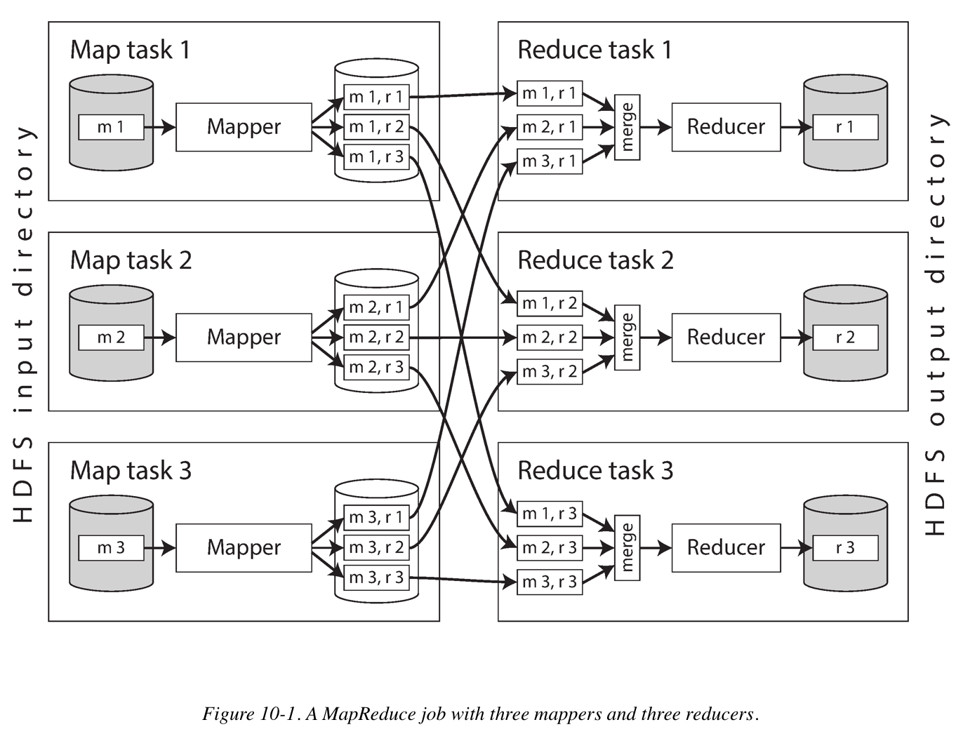
Reduce-Side Joins and Grouping

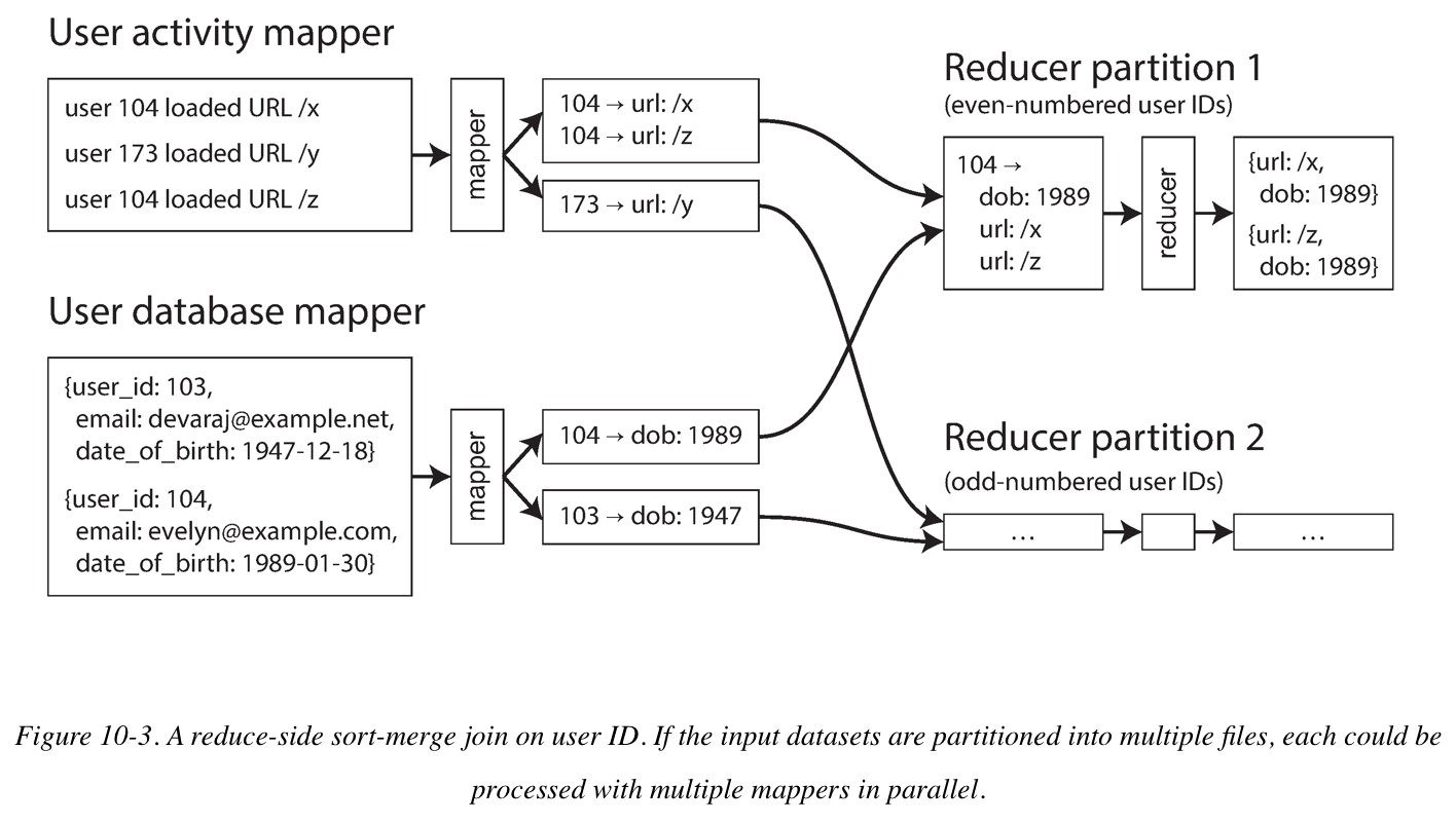
When the MapReduce framework partitions the mapper output by key and then sorts the key-value pairs, the effect is that all the activity events and the user record with the same user ID become adjacent to each other in the reducer input. The Map-Reduce Job can even array the records to be sorted such that the reducer always sees the record from the user database first, followed by the activity events in timestamp order, this technique is know as a secondary sort.

If a join input has hot keys, there are a few algorithms you can use to compensate.

• In Pig, first runs a sampling job to determine which keys are hot. When performing the actual join, the mappers send any records relating to a hot key to one of several reducers, chosen at random (in contrast to conventional hash based). For the other input to the join, records relating to the hot key need to be replicated to all reducers handling that key.

• In Hive, it requires hot keys to be specified explicitly in the table metadata, and it stores records related to those keys in separate files from the rest. When performing a join on that table, it uses a map-side join for the hot keys.

Beyond MapReduce

In response to the difficulty of using MapReduce directly, various high-level programming models (Pig, Hive, Cascading, Crunch) were created as abstractions on top of MapReduce.

Dataflow engines like Spark, Flink, and Tez typically arrange the operators in a job as a directed acyclic graph (DAG). The flow data from one operator to another is structured as a graph, while the data itself typically consists of relational-style tuples.

The two main problems that distributed batch processing frameworks need to resolve are:

• Partitioning

  In MapReduce, mappers are partitioned according to input file blocks, The output of mappers is repartitioned, sorted, and merged into a configurable number of reducer partitions. The purpose of this process is to bring all the related data (e.g., all the records with the same key) together in the same place.

  Post-MapReduce dataflow engines try to avoid sorting unless it is required, but they otherwise take a broadly similar approach to partitioning.

• Fault tolerance

  MapReduce frequently writes to disk, which makes it easy to recover from an individual failed task without restarting the entire job but slows down execution in the failure-free case. Dataflow engines perform less materialization of intermediate state and keep more in memory, which means that they need to recompute more data if a node fails. Deterministic operators reduce the amout of data that needs to be recomputed.

Join Algorithms for MapReduce

• Sort-merge joins

  Each of the inputs being joined goes through a mapper that extracts the join key. By partitioning, sorting, and merging, all the record with the same key end up going to the same call of the reducer. This function can then output the joined records.

• Broadcast hash joins

  One of the two join inputs is small, so it is not partitioned and it can be entirely loaded into a hash table. Thus you can start a mapper for each partition of the large join input, load the hash table for the small input into each mapper, and then scan over the large input one record at a time, querying the hash table for each record.

• Partitioned hash joins

  If the two join inputs are partitioned in the same way (using the same key, same hash function, and same number of partitions), then the hash table approach can be used independently for each partition.

C11 Stream Processing

Streams come from user activity events, sensors, and writes to database, and are transported through direct messaging via message brokers, and in event logs.

Two types of message brokers:

• AMQP/JMS-style message broker

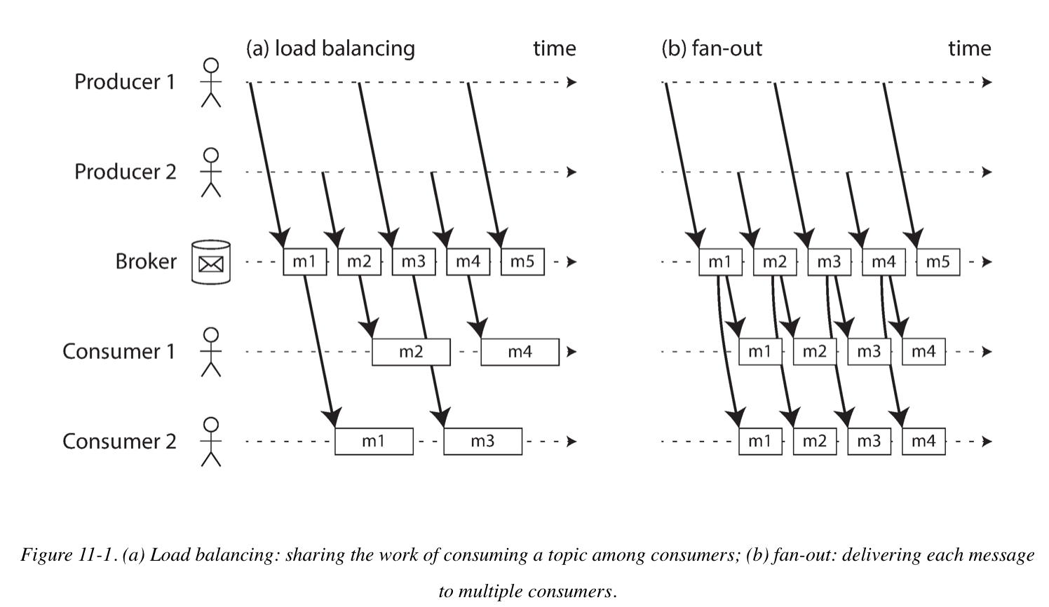
  The broker assigns individual messages to consumers, and consumers acknowledge individual messages when they have been successfully processed. Messages are deleted from the broker once they have been acknowledged. This approach is appropriate as an asynchronous form of RPC. For example in a task queue, where the exact order of message processing is not important and where there is no need to go back and read old messages again after they have been processed.

• Log-based message broker

The broker assigns all messages in a partition to the same consumer node, and always delivers messages in the same order. Parallelism is achieved through partitioning, and consumers track their progress by checkpointing the offset of the last message they have processed. The broker retains messages on disk, so it is possible to jump back and reread old messages if necessary.

Message Brokers and Multiple Producers/Consumers

Message broker is essentially a kind of database that is optimized for handling message streams. It runs as a server, with producers and consumers connecting to it as clients. Producers write messages to the broker, and consumers receive them by reading them from the broker.

When multiple consumers read messages in the same topic, two main patterns of messages are used: Load balancing and Fan-out. They can also be combined: for example, two separate groups of consumers may each subscribe to a topic, such that each group collectively receives all messages, but within each group only one of the nodes receives each messages.

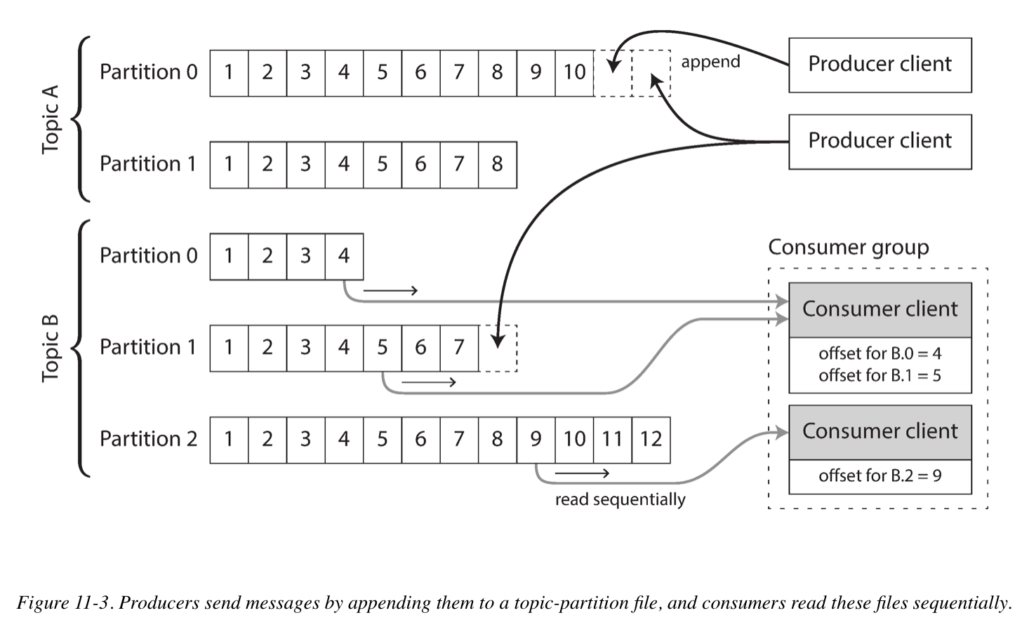
Partitioned logs for message storage

A log is simply an append-only sequence of records on disk. To scale to higher throughput, the log can be partitioned. Different partitions can then be hosted on different machines, making each partition a separate log that can be read and written independently from other partitions.

Within each partition, the broker assigns a monotonically increasing sequence number, or offset, to every message. Such a sequence number makes sense because a partition is append-only, so the messages within a partition are totally ordered.

To reclaim disk space, the log is actually divided into segments, and from time to time old segments are deleted or moved to archive storage. Effectively, the log implements a bounded-size buffer that discards old messages when it gets full, also know as a circular buffer or ring buffer.

In situations where messages may be expensive to process and you want to parallelize processing on a message-by-message basis, and where message ordering is not so important, the JMS/AMQP style of message broker is preferable. On the other hand, in situations with high message throughput, where each message is fast to process and where message ordering is important, the log-based approach works very well.

Change Data Capture

Change Data Capture (CDC) is the process of observing all data changes written to a database and extracting them in a form in which they can be replicated to other systems. CDC is especially interesting if changes are made available as a stream, immediately as they are written.

For example, you can capture the changes in a database and continually apply the same changes to a search index. If the log of changes is applied in the same order, you can expect the data in the search index to match the data in the database. The search index and any other derived data systems are just consumers of the change stream.

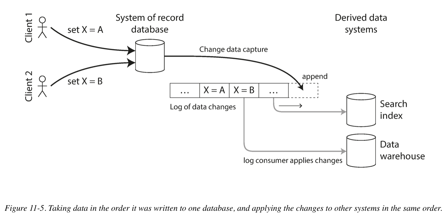
Kafka Connect is an effort to integrate change data capture tools for a wide range of database systems with Kafka. Once the stream of change events is in Kafka, it can be used to update derived data systems. Kafka Connect sinks can export data from Kafka to various different databases and indexes.

Processing Streams

You can process one or more input streams to produce one or more output streams. Streams may go through a pipeline consisting of several such processing stages before they eventually end up at an output.

Several purposes of stream processing, including searching for event patterns (complex event processing), computing windowed aggregations (stream analytics), and keeping derived data systems up to date (materialized views).

Reasoning About Time

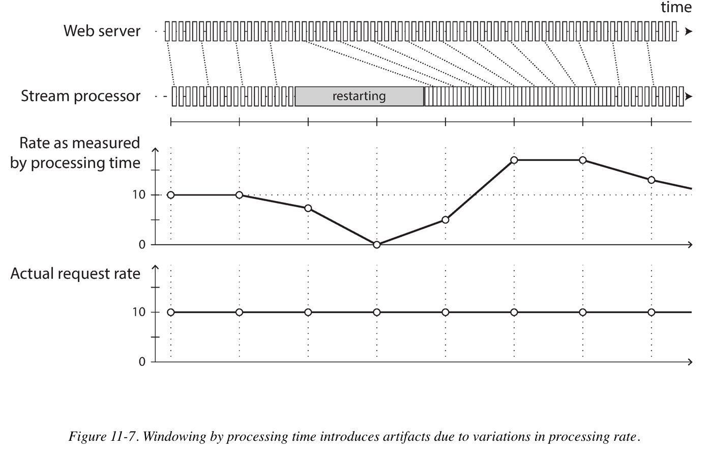
Stream processors often need to deal with time. Confusing event time and processing time leads to bad data. For example, say you have a stream processor that measures the rate of requests. If you redeploy the stream processor, it may be shut down for a minute and process the backlog of events when it comes back up. If you measure the rate based on the processing time, it will look as if there was a sudden anomalous spike of requests while processing the backlog.

Whose clock are we using?

Consider a mobile app that reports events for usage metrics to a server. The app may be used while the device is offline, in which case it will buffer events locally on the device and send them to a server when an internet connection is next available. And the user’s mobile device’s local clock cannot be trusted.

To adjust for incorrect device clocks, one approach is to log three timestamps:

1. The time at which the event occurred, according to the device clock
2. The time at which the event was sent to the server, according to the device clock
3. The time at which the event was received by the server, according to the server clock

By subtracting the second timestamp from the third, you can estimate the offset between the device clock and the server clock. You can then apply the offset to the event timestamp, and thus estimate the true time at which the event actually occurred.

Type of Windows

Tumbling Window

A tumbling window has a fixed length, and every event belongs to exactly one windows. For example, a 1-minute tumbling window could include all events with timestamps between 10:03:00 and 10:03:59. You could implement a 1-minute tumbling window by taking each event timestamp and rounding it down to the nearest minute to determine the window that it belongs to.

Hopping Window

A hopping window also has a fixed length, but allows windows to overlap in order to provide some smoothing. For example, a 5-minute window with a hop size of 1 minute would contain the events between 10:03:00 and 10:07:59, then the next window would cover events between 10:04:00 and 10:08:59, and so on. You can implement this hopping window by first calculating 1-minute tumbling windows, and the aggregating over several adjacent windows.

Sliding Window

A sliding window contains all the events that occur within some interval of each other. For example, a 5-minute sliding window would cover events at 10:03:39 and 10:08:12, because they are less than 5 minutes apart. A sliding window can be implemented by keeping a buffer of events sorted by time and removing old events when they expire from the windows. It can also use a fixed size of counts array and timestamp array together with mod calculation. (See Sliding Window Algorithm)

Session Window

Unlike the other window types, a session window has no fixed duration. Instead, it is defined by grouping together all events for the same user that occur closely together in time, and the window ends when the user has been inactive for some time.

Stream-stream Joins (Window Join)

Say you have a search feature on your website, and you want to detect recent trends in searched-for URLs (Click Through Rate). Every time someone types a search query, you log an event containing the query and results returned. Every time some clicks one of the search results, you log another event recording the click.

NOTE: The click may never come if the user abandons their search, and even if it comes, the time between the search and the click may be highly variables.

To implement this type of join, a stream processor needs to maintain state: for example, all the events that occurred in the last hour, indexed by session ID. Whenever a search event or click event occurs, it is added to the appropriate index, and the stream processor also checks the other index to see if another event for the same session ID has already arrived. If there is a matching event, you emit an even saying which search result was clicked. If the search event expires without you seeing a matching click event, you emit an event saying which search results where not clicked.

...&refid=plgooglecpc&refclickid=d%3Achotel12968742300g108140569633139618273kwd-42050722987%7C9003454&`gclid=EAIaIQobChMIw5O46bal2QIV3I-zCh2KnAe1EAAYASAAEgIDEfD_BwE`&slingshot=1134#/search/hotels/norwalk/1

Fault Tolerance

To achieve fault tolerance and exactly-once semantics in a stream processor. As with batch processing, we need to discard the partial output of any failed tasks. However, since a stream process is long-running and produce output continuously, we can’t simply discard all output. Instead, a finer-grained recovery mechanism can be used, based on microbatching, checkpointing, transactions, or idempotent writes.

Even if an operation is not naturally idempotent, it can often be made idempotent with a bit of extra metadata. For example, when consuming messages from Kafka, every message has a persistent, monotonically increasing offset. When writing a value to an external database, you can include the offset of the message that triggered the last write with the value.

Rebuilding state after a failure

Any stream process that requires state, for example, any windowed aggregations and any tables and indexes used for joins, must ensure that this state can be recovered after a failure.

One option is to keep state in a remote datastore and replicate it. An alternative is to keep state local to the stream processor, and replicate it periodically. When the stream processor is recovering from a failure, the new task can read the replicated state and resume processing without data loss.

C12 The Future of Data Systems

• Updating a derived data system based on an event log can often be made deterministic and idempotent, making it quit easy to recover from faults.

• In the absence of widespread support for a good distributed transaction protocol, I believe that log-based derived data is the most promising approach for integrating different data systems.

• Lambda Architecture In the lambda approach, the stream processor consumes the events and quickly produces an approximate update to view; the batch processor later consumes the same set of events and produces a corrected version of the derived view. The reasoning behind this is that batch processing is simpler and thus less prone to bugs, while stream processors are thought to be less reliable and harder to make fault-tolerant. Moreover, the stream process can use fast approximate algorithms while the batch process uses slower exact algorithms. To unify batch and stream processing in one system requires the following features: The ability to replay historical events through the same processing engine that handles the stream of recent events. like log-based message brokers; Exactly-once semantics for stream processors; Tools for windowing by event time, not by processing time.

• As I said in the Preface, building for scale that you don’t need is wasted effort and may lock you into an inflexible design. In effect, it is a form of premature optimization. The goal of unbundling is not to compete with individual databases on performance for particular workloads; the goal is to allow you to combine several different databases in order to achieve good performance for a much wider range of workloads than is possible with a single piece of software. It’s about breadth, not depth.

• The role of caches, indexes, and materialized views is simple: they shift the boundary between the read path and the write path. They allow use to do more work on the write path, by precomputing results, in order to save effort on the read path.

• Pushing state changes to clients: In order to extend the write path all the way to the end user, we would need to fundamentally rethink the way we build many of these systems: moving away from request/response interaction and toward publish/subscribe dataflow. The advantage of more responsive user interfaces and better offline support would make it worth the effort.

• To achieve exactly-once execution of an operation, we need to make the operation idempotent; this is, to ensure that it has the same effect, no matter whether it is executed once or multiple times. You may need to maintain some additional metadata (such as the set of operation IDs/offset that have updated a value), and ensure fencing (using fencing token) when failing over from one node to another.

• Suppress duplicate requests: To make the operation idempotent through several hops of network communication, it is not sufficient to rely just on a transaction mechanism provided by database. You could generate a unique identifier for an operation (such as a UUID) and include it as a hidden form field in the client application, or calculate a hash of all the relevant form fields to derive the operation ID. And add uniqueness constraint on this unique identifier.

ALTER TABLE requests ADD UNIQUE (request_id);

BEGIN TRANSACTION;

INSERT INTO requests
  (request_id, from_account, to_account, amount)
  VALUES('0286FDB8-D7E1-423F-B40B-792B3608036C', 4321, 1234, 11.00);

UPDATE accounts SET balance = balance + 11.00 WHERE account_id = 1234;
UPDATE accounts SET balance = balance - 11.00 WHERE account_id = 4321;

COMMIT;

• Uniqueness in log-based messaging, For example, in the case of several users trying to claim the same username.
  1. Every request for a username is encoded as a message, and appended to a partition determined by the has of the username.
  2. A stream processor sequentially reads the requests in the log, using a local database to keep track of which username are token. For every request for a username that is available, it records the name as taken and emits a success message to an output stream. For every request for a username that is already taken, it emits a rejection message to an output stream.
  3. The client that requested the username watches the output stream and waits for a success or rejection message corresponding to its request.

  Its fundamental principal is that any writes that may conflict are routed to the same partition and processed sequentially.

• Multi-partition request processing In the traditional approach to databases, executing this transaction would require an atomic commit across all three partitions. However, it turns out that equivalent correctness can be achieved with partitioned logs, and without an atomic commit:

  1. The request to transfer money from account A to account B is given a unique request ID by the client, and appended to a log partition based on the request ID. (To ensure that the payer account is not overdrawn by this transfer, you can additionally have a stream processor, partitioned by payer account number, than maintains account balances and validates transactions. Only valid transactions would then be placed in the request log.)

  2. A stream processor reads the log of requests, For each request message it emits two messages to output streams: a debit instruction to the payer account A (partitioned by A), and a credit instruction to payee account B (partitioned by B). The original request ID is included in those emitted messages.

  3. Further processors consume the streams of credit and debit instructions, deduplicate by end-to-end request ID, and apply the changes to the account balances.

  By breaking down the multi-partition transaction into two differently partitioned stages and using the end-to-end request ID, we have achieved the same correctness property even in the presence of faults, and without using an atomic commit protocol.

• Loosely interpreted constraints: In many business contexts, it is actually acceptable to temporarily violate a constraint and fix it up later by apologizing. It may well be a reasonable choice to go ahead with a write optimistically, and to check the constraint after the fact. (Such as over-booked, over-sold, over-drawn)

• Coordination-avoiding data systems

  1. Dataflow systems can maintain integrity guarantees on derived data without atomic commit, linearizability, or synchronous cross-partition coordination.
  2. Although strict uniqueness constraints require timeliness and coordination, many applications are actually fine with loose constraints that may be temporarily violated and fixed up later. as long as integrity is preserved throughout.

  Such Coordination-avoiding data systems have a lot of appeal: they can achieve better performance and fault tolerance than systems that need to perform synchronous coordination. For example, such a system could operate distributed across multiple datacenters in a multi-leader configuration, asynchronously replicating between regions. Any one datacenter can continue operation independently from the others.

  By structuring application around dataflow and checking constraints asynchronously, we can avoid most coordination and create systems that maintain integrity but still perform well, even in geographically distributed scenarios and in the presence of faults.

• Doing the Right Thing

A technology is not good or bad in itself – what matters is how it is used and how it affects people. The ethical responsibility is our engineers to bear also.

Having privacy does not mean keeping everything secret; it means having the freedom to choose which things to reveal to who, what to make public, and what to keep secret. The right to privacy is a decision right: it enables each person to decide where they want to be on the spectrum between secrecy and transparency in each situation.

As software and data are having such a large impact on the word, we engineers must remember that we carry a responsibility to work toward the kind of work that we want to live in: a world that treats people with humanity and respect. I hope that we can work together toward that goal.

Reference Resources

• Martin Kleppmann: “Design Data-Intensive Applications”, March 2017