Database Topics
Indexing
-
An index is a data structure, mostly a B-tree which is time efficient (lookup, deletion, insertion) can all be done in logarithmic time, also it’s sorted inside, helpful for range lookup: like find out all of the employees who are less than 40 years old.
-
An index stores the value of indexed column, and also pointers to the corresponding rows in the table, something like (“Jesus”, 0x82829). There are Clustered and Non-clustered indexes.
-
A clustered index is a special type of index that reorders the way records in the table are physically stored. Therefore table can have only one clustered index. The leaf nodes of a clustered index contain the data pages; A non-clustered index is a special type of index in which the logical order of the index does not match the physical stored order of the rows on disk. The leaf node of a non-clustered index does not consist of the data pages. Instead, the leaf nodes contain index rows.
-
Other types of indexes: Hash index, R-tree, Bitmap index.
Deadlock
In databases avoid making lots of changes to different tables in a single transaction, avoid triggers and switch to optimistic/dirty/nolock reads as much as possible.
With multi-threads case, make sure you change the different sets of data in the same table in each thread; the deadlock could be triggered if the parallel threads are trying to read & write the overlapped data/tables at the same time.
Stored Procedure
- How to use stored procedure and return result set?
SQL> create procedure myproc (prc out sys_refcursor)
  2  is
  3  begin
  4     open prc for select * from emp;
  5  end;
  6  /

Procedure created.

SQL> var rc refcursor
SQL> execute myproc(:rc)

PL/SQL procedure successfully completed.

SQL> print rc

     EMPNO ENAME      JOB              MGR HIREDATE           SAL       COMM     DEPTNO
---------- ---------- --------- ---------- ----------- ---------- ---------- ----------
      7839 KING       PRESIDENT            17-NOV-1981       4999                    10
      7698 BLAKE      MANAGER         7839 01-MAY-1981       2849                    30
      7782 CLARKE     MANAGER         7839 09-JUN-1981       2449                    10
JDBC Performance Tips
- Use Cache, reduce many calls.
- Use Database Index, (might slow down insert and update).
- Use Prepared Statement, use parameterized sql queries.
- Use Database Connection Pool
- Use JDBC Batch Update, use executeBatch()
- Disable Auto Commit
- Use IN with 3000 limit
- Pagination and Multi-threads
- Not use ORM (Object/Relational Mapping) framework, or JPA implementation
Access Hadoop with Hive Driver
public DataSource dataSourceTrafficCop() throws Exception {
  String dbHive = Constants.getStr("db.trafficcop");
  logger.info("Connecting Hive TrafficCop Data Source {}...", dbHive);
  // System.setProperty("java.security.krb5.conf", "/apps/home/eng/kerberos/krb5.conf");
  System.setProperty("java.security.krb5.conf", Constants.getStr("java.security.krb5.conf", "/apps/home/eng/kerberos/krb5.conf"));
  org.apache.hadoop.conf.Configuration conf = new org.apache.hadoop.conf.Configuration();
  conf.set("hadoop.security.authentication", "kerberos");
  UserGroupInformation.setConfiguration(conf);
  String username = Constants.getStr("kerberos.hadoop.username", "archer/archer@UNIX.PCLN.COM");
  String keytabFile = Constants.getStr("kerberos.hadoop.keytab", "/apps/home/eng/kerberos/archer.service.keytab");
  UserGroupInformation.loginUserFromKeytab(username, keytabFile);

  SimpleDriverDataSource dataSource = new SimpleDriverDataSource();
  dataSource.setDriverClass(HiveDriver.class);
  dataSource.setUrl(Config.getStr(dbHive, "DBURL"));

  return dataSource;
}
Oracle Database
Table Partitions
- This following sample partitioned the table by
DayandID.
CREATE TABLE SEM.META_PERF_ALL_METRIC
(
   ACTIVITY_DATE DATE NOT NULL,
   PARTNER_ID NUMBER NOT NULL,
   PARTNER_NAME VARCHAR2(16 BYTE),
   ......
   CREATION_DATE_TIME DATE,
   MOD_DATE_TIME DATE,
   SYNC_ID NUMBER
)
TABLESPACE T_SEM
PARTITION BY RANGE (ACTIVITY_DATE)
   INTERVAL ( NUMTODSINTERVAL(1, 'DAY') )
   SUBPARTITION BY LIST (PARTNER_ID)
      SUBPARTITION TEMPLATE(SUBPARTITION BENGHA VALUES ('1'),
                            SUBPARTITION BENTRV VALUES ('2'),
                            SUBPARTITION UNKNOWN VALUES ('-1'))
   (PARTITION P_META_PERF_ALL_01
       VALUES LESS THAN (TO_DATE('2016-01-01', 'YYYY-MM-DD'))
       TABLESPACE T_SEM
       (SUBPARTITION P_META_PERF_ALL_01_BENGHA VALUES ('1') TABLESPACE T_SEM,
        SUBPARTITION P_META_PERF_ALL_01_BENTRV VALUES ('2') TABLESPACE T_SEM,
        SUBPARTITION P_META_PERF_ALL_01_UNKNOWN VALUES ('-1') TABLESPACE T_SEM));
- In favor of dropping partition efficiently, better use local index
CREATE TABLE SEM.META_CHANGESET_BID
(
   CHANGESET_BID_ID NUMBER NOT NULL,
   CHANGESET_ID NUMBER NOT NULL,
   PARTNER_NAME VARCHAR2(32 BYTE),
   ACCOUNT_NAME VARCHAR2(128 BYTE),
   ......
   PROCESS_STATUS_ID NUMBER,
   ERROR_MESSAGE VARCHAR2(512 BYTE),
   CREATION_DATE_TIME DATE DEFAULT SYSDATE NOT NULL
)
TABLESPACE T_SEM
PARTITION BY RANGE
   (CREATION_DATE_TIME)
   INTERVAL ( NUMTODSINTERVAL(1, 'DAY') )
   (PARTITION P_META_CHANGESET_BID_01 VALUES LESS THAN (TO_DATE('2017-04-01', 'YYYY-MM-DD')) TABLESPACE T_SEM);


CREATE INDEX SEM.IDX_META_CHGSET_BID_CHGSET_ID
   ON SEM.META_CHANGESET_BID(CHANGESET_ID)
   TABLESPACE I_SEM
   LOCAL (PARTITION P_META_CHANGESET_BID_01 TABLESPACE I_SEM);
- Query from a specified partition
SELECT hotel_id, pos, DECODE(device, 'WEB', 'DESKTOP', device) AS device
  FROM meta_perf_all_metric PARTITION FOR(TO_DATE('08/13/2017', 'MM/DD/YYYY'))
 WHERE partner_id = 9;
- Oracle Optimizer Hints
leading(e j), index(), append, parallel(4), use_hash(ca,rs), full(a)
MERGE
INTO         sem_adgroup_criterion cc
using        (
                    SELECT x.adgroup_criterion_id,
                           x.criterion_id,
                           c.criterion_id AS new_criterion_id
                    FROM   (
                                  SELECT
                                         /*+ leading(cr) */
                                         cc.adgroup_criterion_id,
                                         cc.criterion_id,
                                         cr.partner_criterion_id
                                  FROM   sem_adgroup_criterion cc
                                  JOIN   sem_criterion cr
                                  ON     cr.search_id = 1
                                  AND    cr.criterion_type_id = 20
                                  AND    cr.criterion_id = cc.criterion_id
                                  JOIN   sem_adgroup g
                                  ON     cc.adgroup_id = g.adgroup_id
                                  JOIN   sem_campaign c
                                  ON     g.campaign_id = c.campaign_id
                                  WHERE  c.account_id = ? ) x,
                           sem_criterion c
                    WHERE  c.search_id = ?
                    AND    c.criterion_type_id = 20
                    AND    x.partner_criterion_id = c.partner_criterion_id) rs
ON (
                          cc.adgroup_criterion_id = rs.adgroup_criterion_id )
WHEN matched THEN
UPDATE
SET    cc.criterion_id = rs.new_criterion_id
Spatial Database
A spatial database is a database that is optimized for storing and querying data that represents objects defined in a geometric space. It uses a spatial index to speed up database operations.
R-tree is typically the preferred method for indexing spatial data. Objects (shapes, lines and points) are grouped using the minimum bounding rectangle (MBR). Objects are added to an MBR within the index that will lead to the smallest increase in its size.
MBRs are frequently used as an indication of the general position of a geographic feature or dataset, for either display, first-approximation spatial query, or spatial indexing purposes.
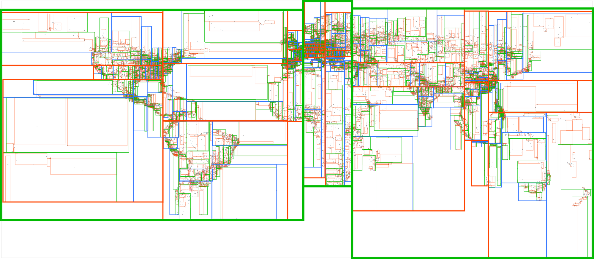
A visualization of an R-tree for 138k populated places on Earth
Spatial Search Algorithm
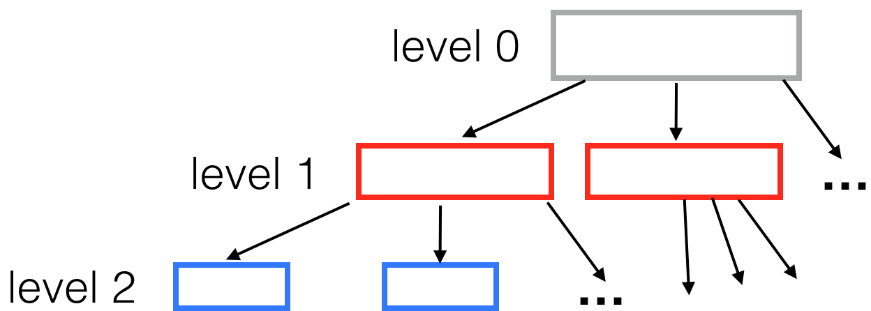
Spatial data has two fundamental query types: nearest neighbors and range queries. Solving both problems at scale requires putting the points into a spatial index. Almost all spatial data structures share the same principle to enable efficient search: branch and bound. It means arranging data in a tree-like structure that allows discarding branches at once if they do not fit our search criteria.
Let’s see how to build a R-tree. we start with a bunch of input points and sort them into 9 rectangular boxes with about the same number of points in each. We’ll repeat the same process a few more times until the final boxes contain 9 points at most. Besides points, R-tree can contain rectangles, which can in turn represent any kinds of geometric objects. It can also extend to 3 or more dimensions.
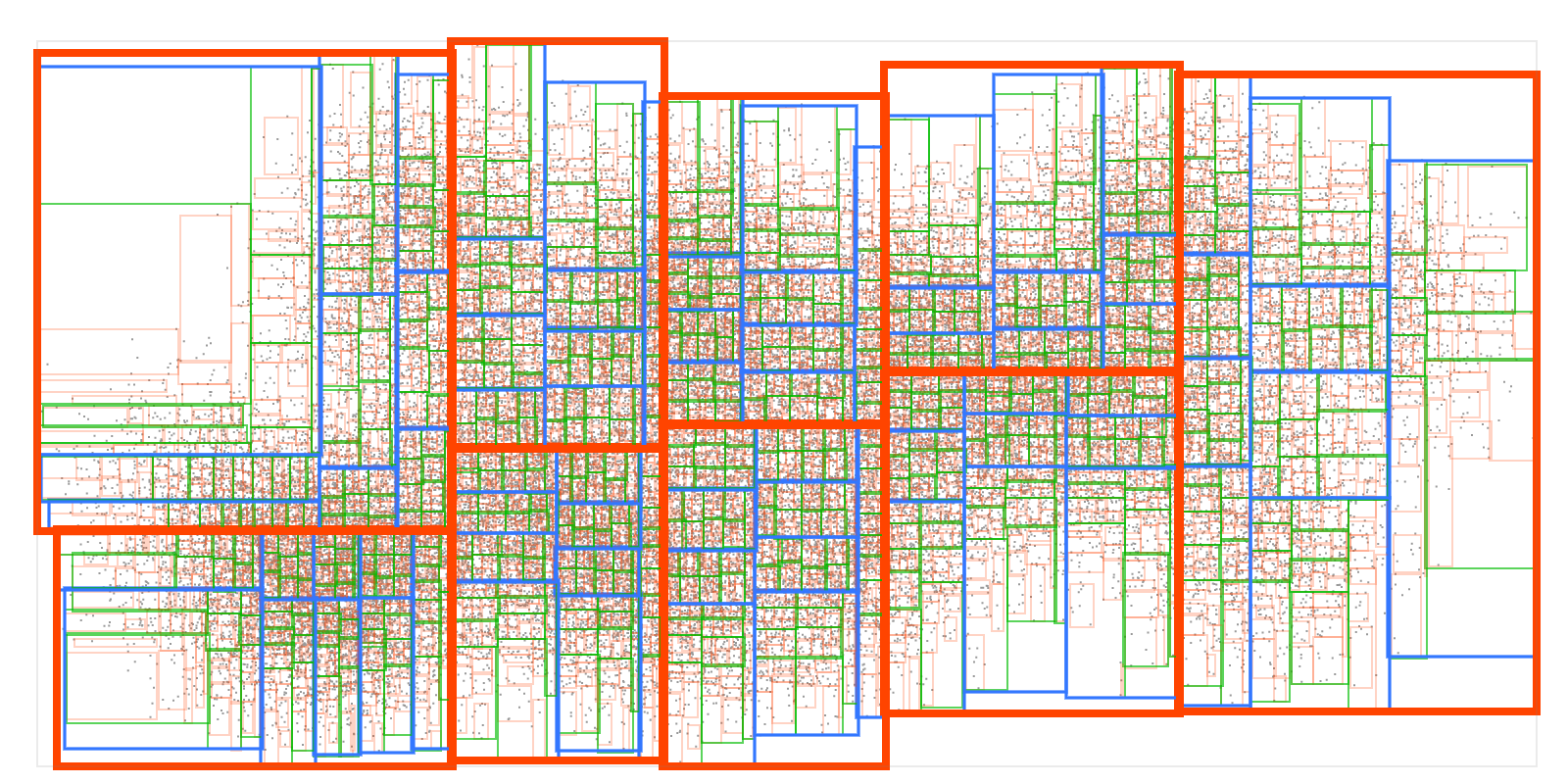
Each node has a fixed number of children (in our R-tree example, 9). How deep is the resulting tree? For one million points, the tree height will equal ceil(log(1000000) / log(9)) = 7. When performing a range search on such a tree, we can start from the top tree level and drill down, ignoring all the boxes that don’t intersect our query box. For a small query box, this means discarding all but a few boxes at each level of the tree. So getting the results won’t need much more than sixty box comparisons (7 * 9 = 63) instead of a million. Making it ~16000 times faster than a naive loop search in this case. So the time complexity is O(Klog(N)) where K is the number of results.
To search a spatial tree for nearest neighbors, we’ll take advantage of another neat data structure — a priority queue. It allows keeping an ordered list of items with a very fast way to pull out the “smallest” one. We start our search at the top level by arranging the biggest boxes into a queue in the order from nearest to farthest. Next, we “open” the nearest box, removing it from the queue and putting all its children (smaller boxes) back into the queue alongside the bigger ones. We go on like that, opening the nearest box each time and putting its children back into the queue. When the nearest item removed from the queue is an actual point, it’s guaranteed to be the nearest point. The second point from the top of the queue will be second nearest, and so on.